You might consider some of the following:
data = {{100, 20, 0.1}, {120, 20, 0.12}, {140, 20, 0.15}, {160, 20, 0.18}, {180, 20, 0.24},
{200, 20, 0.37}, {100, 40, 0.3}, {120, 40, 0.35}, {140, 40, 0.38}, {160, 40, 0.42},
{180, 40, 0.48}, {200, 40, 0.54}, {100, 60, 0.6}, {120, 60, 0.63}, {140, 60, 0.68},
{160, 60, 0.72}, {180, 60, 0.78}, {200, 60, 0.84}};
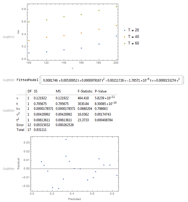
(* Plot the data *)
ListPlot[{data[[{1, 2, 3, 4, 5, 6}, {1, 3}]],
data[[{7, 8, 9, 10, 11, 12}, {1, 3}]],
data[[{13, 14, 15, 16, 17, 18}, {1, 3}]]},
Frame -> True, FrameLabel -> {"v", "mu"},
PlotLegends -> {"T = 20", "T = 40", "T = 60"}]
(* Fit linear model *)
lm = LinearModelFit[data, {v, t, v *t, v^2, t^2}, {v, t}]
(* Show ANOVA table *)
lm["ANOVATable"]
(* Plot residuals *)
ListPlot[Transpose[{lm["PredictedResponse"], lm["FitResiduals"]}],
Frame -> True, FrameLabel -> {"Predicted", "Residual"}]
resulting in the following output: