Message Boards Message Boards

The Chaos Game - Sierpinski triangles and beyond - part I

EDIT: See also the follow up posts here. and here.
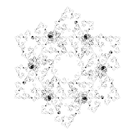
enter image description here

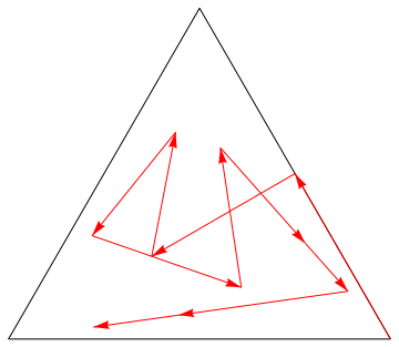
Roughly 8-9 years ago a friend of mine told me I could make the Sierpinski triangle by starting at one of the vertices of an equilateral triangle, and then repeatedly jump half-way to one of the (randomly chosen) vertices.

0 memory

The following code will accomplish that:

ClearAll[sequence]
sequence[n_,m_]:=RandomChoice[Range[n],m]
pts=N@CirclePoints[3];
pts=FoldList[(#1+pts[[#2]])/2&,RandomChoice[pts],sequence[3,10]]
Graphics[{{FaceForm[],EdgeForm[Black],RegularPolygon[3]},Red,Arrow[Partition[pts,2,1]]}]

giving:
enter image description here

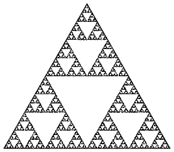
If one does this 1000s of time, and only mark the viewed points, one will get:

ClearAll[sequence]
sequence[n_,m_]:=RandomChoice[Range[n],m]
pts=N@CirclePoints[3];
pts=FoldList[(#1+pts[[#2]])/2&,RandomChoice[pts],sequence[3,25000]];
Graphics[{FaceForm[],EdgeForm[Black],RegularPolygon[3],PointSize[0.001],Point[pts]}]

giving:
enter image description here

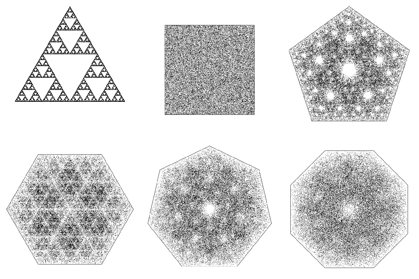
Which will indeed show that by randomly choosing a vertex we can still get structure! Quite a surprise! Of course we can do this with squares, pentagons, hexagons et cetera:

ClearAll[sequence]
sequence[n_,m_]:=RandomChoice[Range[n],m]
Table[
    circlepoints=N@CirclePoints[n];
    pts=FoldList[(#1+circlepoints[[#2]])/2&,RandomChoice[circlepoints],sequence[n,50000]];
    Rasterize[Graphics[{FaceForm[],EdgeForm[Black],RegularPolygon[n],PointSize[0.001],Point[pts]},ImageSize->500,PlotRange->1.1],"Image"]
,
    {n,3,8}
] // Partition[#, 3] & // ImageAssemble

giving:
enter image description here

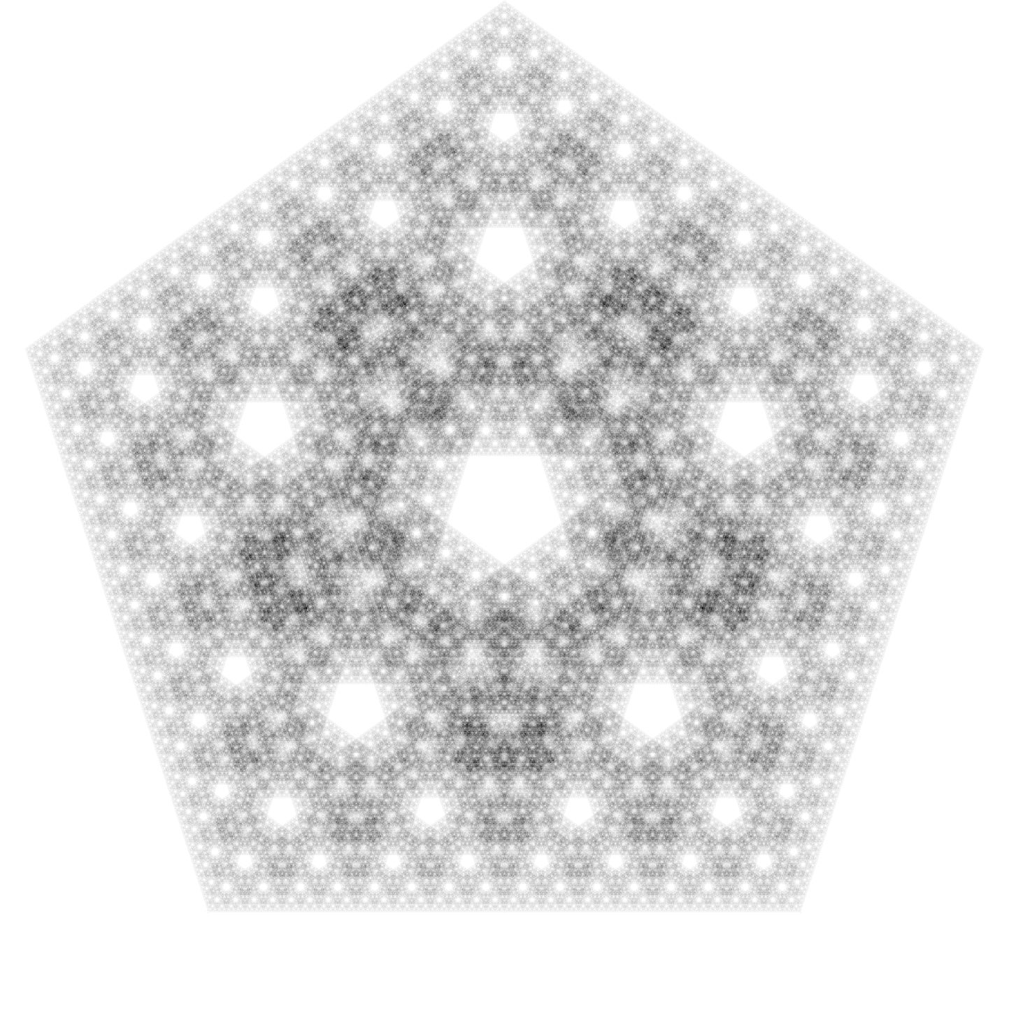
Very neat! (apart from 4, which just gives a homogeneous distribution of points). Here I run the pentagon many many points and high resolution to get:
enter image description here

Where now the gray-color represents the density of points.

0 memory - restricted

Now we can make the dynamics a bit more interesting by not moving to any other vertex but to only specific vertices. Imagine that we are at some position p, then we always have n choices (n being the number of sides): we can jump to the vertex 1 ahead, 2 ahead, .... n ahead (same as last time).

ClearAll[CreateSequence,CreateSequenceImage]
CreateSequence[n_,steps_,choices_]:=Mod[Accumulate[RandomChoice[choices,steps-1]~Prepend~1],n,1]
CreateSequenceImage[n_,m_,choices_]:=Module[{seq,pts},
    seq=CreateSequence[n,m,choices];
    pts=N@CirclePoints[n];
    seq=FoldList[(#1+pts[[#2]])/2&,First[pts],seq];
    Rasterize[Graphics[{PointSize[0.001],Point[seq]},ImageSize->500,PlotRange->1],"Image",RasterSize->{300,300}]
]

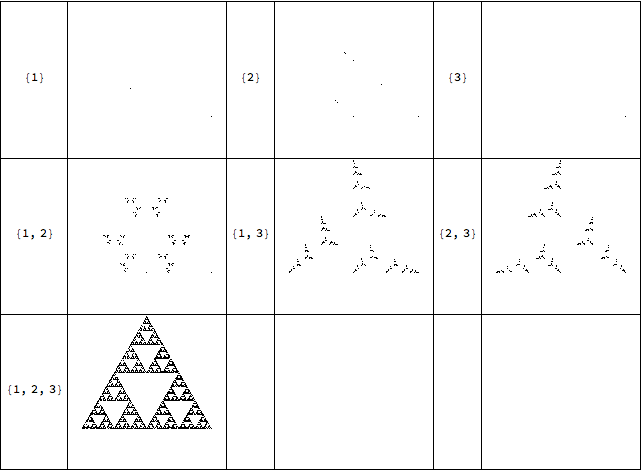
For a 3 sided polygon (i've been told these are called triangles) we can jump 1, 2, or 3 ahead or subsets of that:

Grid[Join@@@Partition[{#,CreateSequenceImage[3,10^5,#]}&/@Subsets[Range[3],{1,\[Infinity]}],UpTo[3]],Frame->All]
enter image description here

Some interesting structure can be seen for some of the subsets.

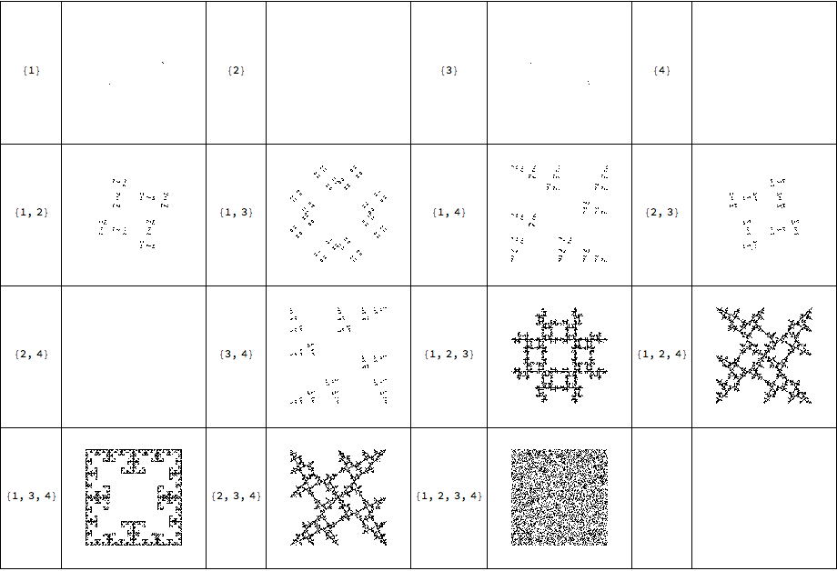
For squares:

Grid[Join@@@Partition[{#,CreateSequenceImage[4,10^5,#]}&/@Subsets[Range[4],{1,\[Infinity]}],UpTo[4]],Frame->All]
enter image description here

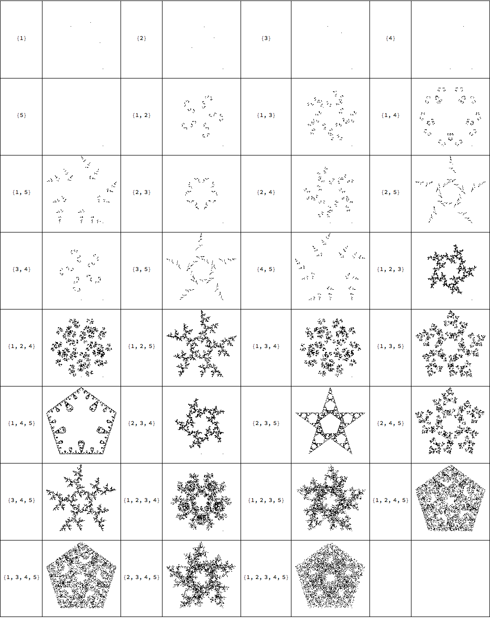
and for pentagons:

Grid[Join@@@Partition[{#,CreateSequenceImage[5,10^5,#]}&/@Subsets[Range[5],{1,\[Infinity]}],UpTo[4]],Frame->All]
enter image description here

the higher the number of sides, the more subsets we can choose. The number of subsets scales as 2^n -1 (minus one because the set can not be empty; we have to jump somewhere!).

Lastly, for hexagons:

Grid[Join@@@Partition[{#,CreateSequenceImage[5,10^5,#]}&/@Subsets[Range[5],{1,\[Infinity]}],UpTo[4]],Frame->All]
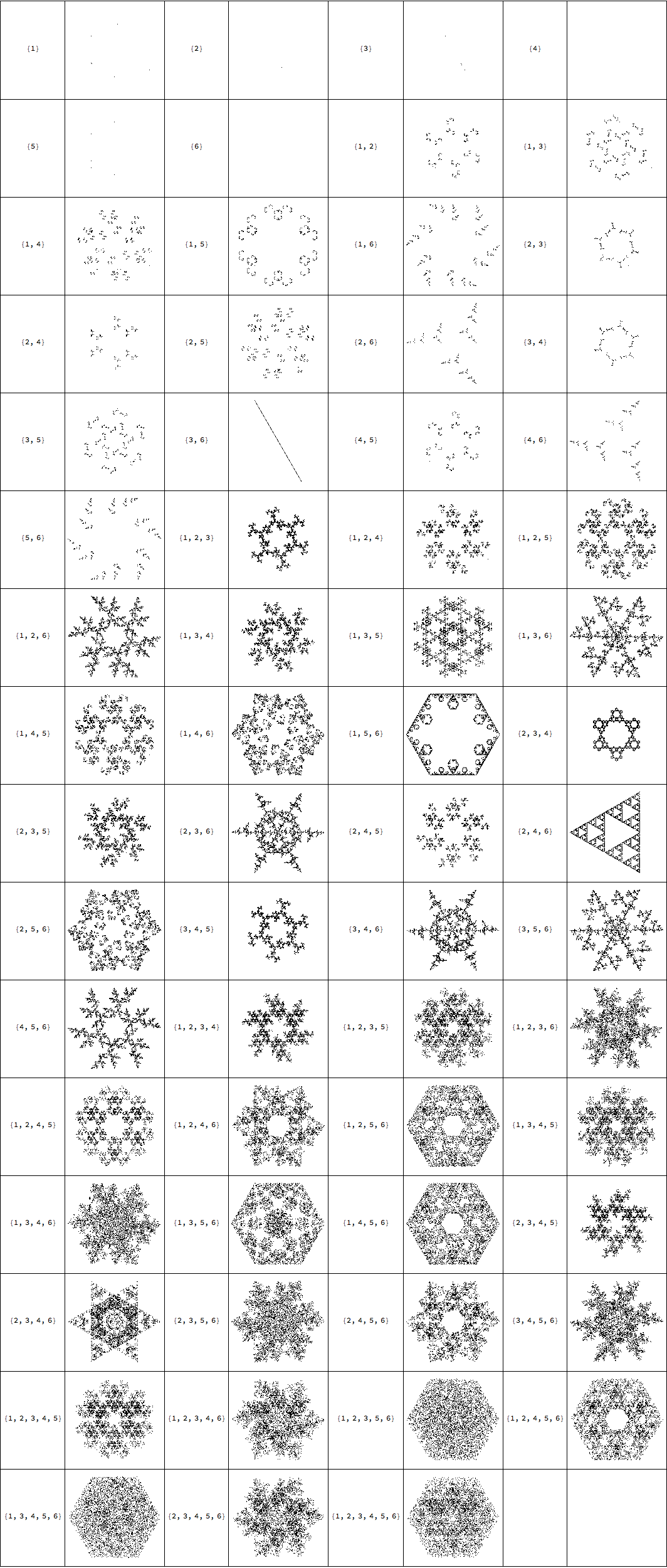
enter image description here

Ok, you can try polygons with large number of sides on your own, but note that the number of subsets doubles every time.

1 memory - restricted

We can even go beyond this, and consider the position of the penultimate vertex as well:
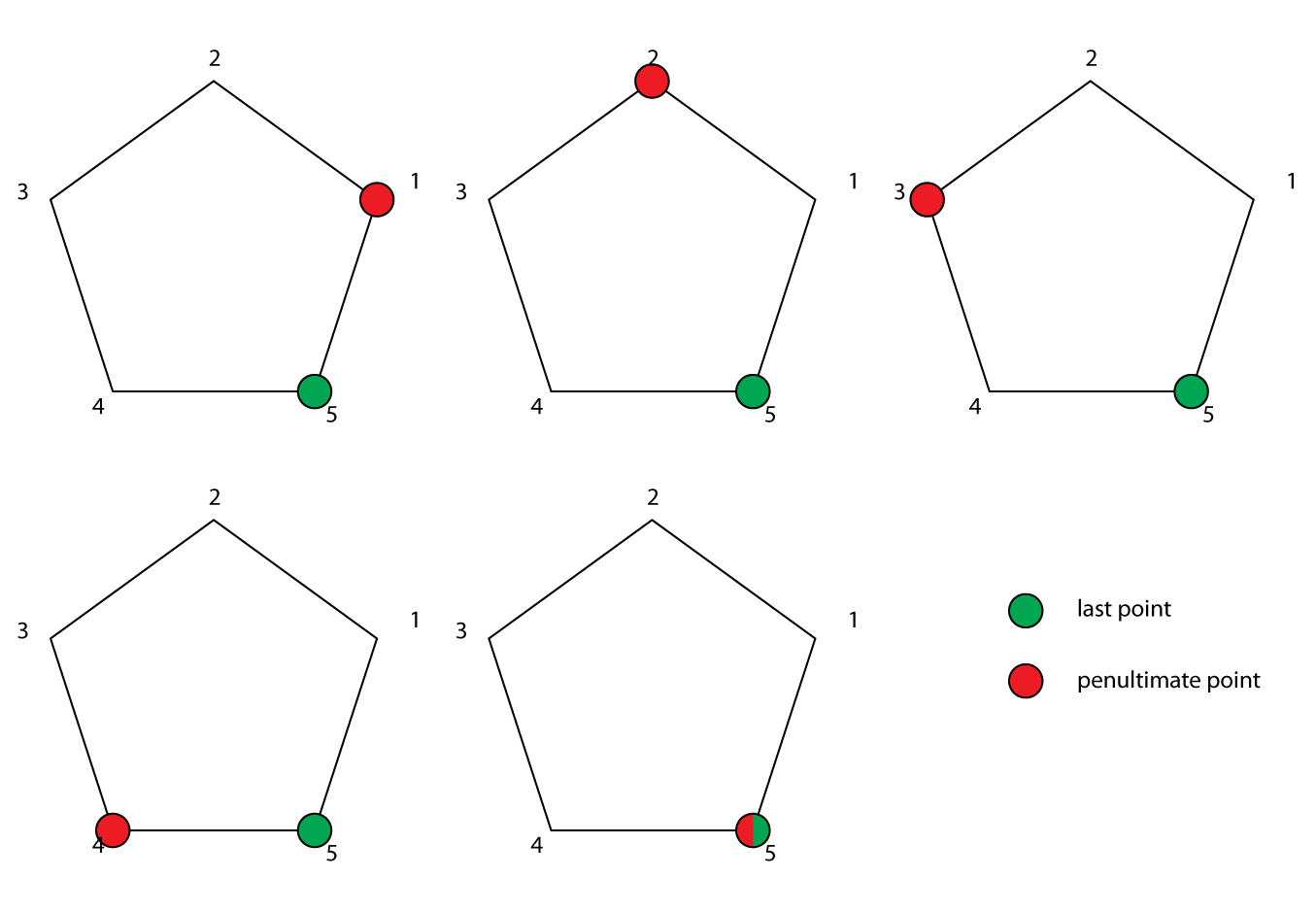
enter image description here

We can consider 5 cases for a pentagon (or, in general, n cases). We will consider the last point to be at position 0 (or n), now the penultimate vertex could be in 5 different positions. For each of these combinations we can choose a different subset of {1,2,3,4,5}. Just to get an idea how many possibilities we now have:

the number of subsets is 2^n - 1, and we have to choose n of these, so there will be (2^n-1)^n different systems to explore:

Table[{n, (2^n - 1)^n}, {n, 3, 8}] // Grid
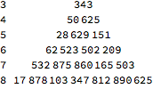
enter image description here

as one can see, the combination grow very quickly.

ClearAll[Stamp,CreateSequence2,CreateSequenceImage2]
CreateSequence2[n_,m_,start:{start1_,start2_},choices_]:=Module[{out,last, penultimate,new,pos2},
    {penultimate,last}=out=start;
    out=Reap[Do[
        pos2=Mod[penultimate-last,n,1];
        new=Mod[last+RandomChoice[choices[[pos2]]],n,1];
        penultimate=last;
        last=new;
        Sow[new]
    ,
        {m-2}
    ]][[2,1]];
    Join[start,out]
]
Stamp[n_,choices_]:=Module[{},
    Image[Normal[SparseArray[Thread[Join@@MapThread[Thread[{#1,#2}]&,{Range[Length[choices]],choices}]->1],{n,n}]]]
]
CreateSequenceImage2[n_,m_,start:{start1_,start2_},choices_]:=Module[{seq,pts,ras,stamp},
    seq=CreateSequence2[n,m,start,choices];
    pts=N@CirclePoints[n];
    seq=FoldList[(#1+pts[[#2]])/2&,First[pts],seq];
    ras=Rasterize[Graphics[{PointSize[0.001],Point[seq]},ImageSize->500,PlotRange->1],"Image",RasterSize->{300,300}];
    stamp=ImagePad[Stamp[n,choices],1,Red];
    ImageCompose[ras,stamp,{Center,Bottom},{Center,Bottom}]
]

Before looking at the general case, we can look at a small subset, namely one can not jump i ahead from the last, and j ahead from the penultimate. Here the example for i=1, and j =3:

ClearAll[JumpPos2]
JumpPos2[n_,{d1_,d2_}]:=Module[{pos},
    pos=Range[n];
    pos=DeleteCases[pos,d1];
    DeleteCases[pos,Mod[d2+#,n,1]]&/@Range[n]
]
CreateSequenceImage2[4,10^4,{1,2},JumpPos2[4,{1,3}]]
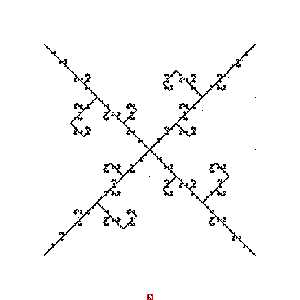
enter image description here

Very neat structure! Of course we can try all i and j from the set {1,2,3,4}:

delta=Tuples[Range[4],2];
deltas=JumpPos2[4,#]&/@delta;
Grid[Join@@@Table[{{i,j},CreateSequenceImage2[4,10^4,{1,2},JumpPos2[4,{i,j}]]},{i,4},{j,4}],Frame->All]
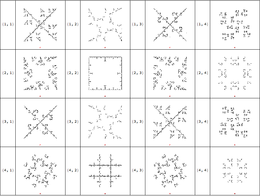
enter image description here

All very neat, but it is just a small subset of the 50625 possibilities. Here let's try 64 random ones:

sc=Reverse@Subsets[Range[4],{1,\[Infinity]}];
Table[
   CreateSequenceImage2[4,10^4,{1,2},RandomChoice[sc,4]]
,
    {64}
] // Partition[#,8]& // ImageAssemble
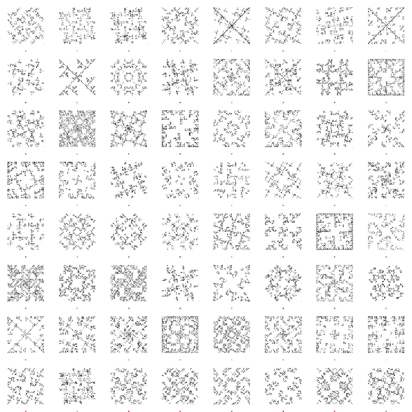
enter image description here

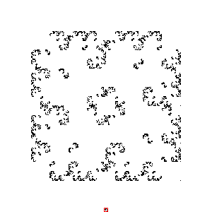
As you can see very nice and rich structure! Notice that I 'stamped' all of them with their 'input':

CreateSequenceImage2[4, 10^4, {1, 2}, {{1, 4}, {3}, {1, 3, 4}, {1, 2, 3}}]
enter image description here

And if one looks closely (save the image and zoom), one will see the 'stamp' (or the rule) at the bottom:

enter image description here

This can be read as follows:

  • The first (top) line, the white pixels are in places 1 and 4, so if the penultimate vertex was '1', move 1 or 4 places from the last vertex
  • The 2nd line, the white pixel is in place 3, jump the position 3 ahead compared to last vertex
  • 3rd line, white pixel at 1,3, and 4.
  • 4th line 1, 2, or 3.

Basically the nth line corresponds to the position of the penultimate vertex. and the white pixels corresponds to 'allowed' number of jumps.

I'll stop here for now. There are many more ideas to explore, I'll name a few:

  • 3D positions, 3D images See below the post of Henrik!
  • Anything other than regular polygons
  • Have different probabilities for each of the vertices...
  • Move in the perpendicular direction
  • ...

See also the follow up posts here. and here and some additional visualizations below!

POSTED BY: Sander Huisman
12 Replies

The functionality of this post has been summarized in the function GeneralizedChaosGame, available on the Wolfram Function Repository:

https://resources.wolframcloud.com/FunctionRepository/resources/GeneralizedChaosGame

So you can now try this out using simply:

ResourceFunction["GeneralizedChaosGame"][3, 3 10^4]

Enjoy!

POSTED BY: Sander Huisman

enter image description here - Congratulations! This post is now Staff Pick! Thank you for your wonderful contributions. Please, keep them coming!

POSTED BY: EDITORIAL BOARD

Thanks!

POSTED BY: Sander Huisman

Dear Sander,

brilliant - as always! I already knew the 'chaos game', but I was not aware of the fact that it works with simple points - I would have tried something using a sub-triangular mapping ... Thank you very much for sharing!

I could not resist trying your method in 3D! Unfortunately this is much less spectacular ...

ClearAll["Global`*"]
sequence[n_, m_] := RandomChoice[Range[n], m]

fromSphericalCoordinates[{r_, \[Theta]_, \[Phi]_}] := 
  FromSphericalCoordinates[{r, \[Theta], \[Phi]}];
fromSphericalCoordinates[{1, 0., _}] = {0, 0, 1};

sphereDist[sph1_, sph2_] := 
 EuclideanDistance[fromSphericalCoordinates[Prepend[sph1, 1]], 
  fromSphericalCoordinates[Prepend[sph2, 1]]]

(* calculates n positions on a 3D-sphere with minimal 'energy' when \
repulsive  *)

sphereAewquiDist[n_Integer /; n > 2] := 
 Module[{vars, vpairs, energy, constr, sol},
  vars = (({Subscript[\[Theta], #1], Subscript[\[Phi], #1]} &) /@ 
     Range[n]); vpairs = Subsets[vars, {2}]; 
  energy = Total[1./Apply[sphereDist, vpairs, {1}]];
  constr = 
   Flatten[Apply[{0 <= #1 <= Pi, -Pi <= #2 <= Pi} &, vars, {1}]];
  sol = Last[NMinimize[{energy, constr}, constr[[All, 2]]]]; 
  Chop[fromSphericalCoordinates /@ (vars /. 
       sol /. {\[Theta]_, \[Phi]_} :> {1, \[Theta], \[Phi]})]]

gr = Table[
   sPts = sphereAewquiDist[n];
   chmLines = MeshPrimitives[ConvexHullMesh[sPts], 1];
   pts = FoldList[(#1 + sPts[[#2]])/2 &, RandomChoice[sPts], 
     sequence[n, 500000]];
   {n, Graphics3D[{Black, Thick, chmLines, Blue, PointSize[0.0001], 
      Point[pts]}, AspectRatio -> Automatic, ImageSize -> 600, 
     SphericalRegion -> False, Boxed -> False]},
   {n, 4, 6}];

Grid[gr, Frame -> All]

The result:

enter image description here

Best regards -- Henrik

POSTED BY: Henrik Schachner

Wow! Very nice Henrik! For 4 this is a tetrahedron and for 6 an octahedron right? For 5; I have no idea what that is called! For the case of 4 you can see the 3D Sierpinski quite nicely. For the others I think the visualisation is the problem; there seems to be some structure, but hard to figure out how it is shaped! I like your sphereAewquiDist function; the future will be bright for you! That is all I can say!

POSTED BY: Sander Huisman

@Henrik Schachner Since it is now public knowledge: https://reference.wolfram.com/language/ref/SpherePoints.html SpherePoints will be introduced in version 11.1 which is similar to your sphereAewquiDist function, with some hard-coded position for 'small' n. and for large 'n' a fast procedure.

POSTED BY: Sander Huisman

Dear Sander,

thank you for this interesting detail! It is a good thing if there is a specific function for this, because my feeling is that my "solution" (turning it into an optimization problem) is quite inappropriate. My little procedure originally stems from the task of finding "equally spaced" beam directions in radiotherapy.

Best regards -- Henrik

POSTED BY: Henrik Schachner

Just as a minor addendum:

From the documentation:

SpherePoints[n] gives the positions of n uniformly distributed points on the surface of a unit sphere.

At least for certain small numbers of points I would not regard this function as "working". See the following examples using 10, 11 and 13 points (left: result of SpherePoints - right: more like expected result):

enter image description here

This is somewhat disappointing. My code for the above:

ClearAll["Global`*"]

fromSphericalCoordinates[{r_, \[Theta]_, \[Phi]_}] := 
  FromSphericalCoordinates[{r, \[Theta], \[Phi]}];
fromSphericalCoordinates[{1, 0., _}] = {0, 0, 1};
sphereDist[sph1_, sph2_] := 
 EuclideanDistance[fromSphericalCoordinates[Prepend[sph1, 1]], 
  fromSphericalCoordinates[Prepend[sph2, 1]]]

mySpherePoints[n_Integer /; n > 2] := 
 Module[{vars, vpairs, energy, constr, sol}, 
  vars = (({Subscript[\[Theta], #1], Subscript[\[Phi], #1]} &) /@ 
     Range[n]); vpairs = Subsets[vars, {2}];
  energy = Total[1./Apply[sphereDist, vpairs, {1}]];
  constr = 
   Flatten[Apply[{0 <= #1 <= Pi, -Pi <= #2 <= Pi} &, vars, {1}]];
  sol = Last[NMinimize[{energy, constr}, constr[[All, 2]]]];
  Chop[fromSphericalCoordinates /@ (vars /. 
       sol /. {\[Theta]_, \[Phi]_} :> {1, \[Theta], \[Phi]})]]

GraphicsGrid[(Show[
       Graphics3D[{Opacity[.3], Sphere[]}, SphericalRegion -> True], 
       ConvexHullMesh[#]] & /@ {SpherePoints[#], 
      mySpherePoints[#]}) & /@ {10, 11, 13}, Frame -> All, 
 ImageSize -> 600]

Regards -- Henrik

POSTED BY: Henrik Schachner

10 and 11 (among others) are hard-coded:

Cases[DownValues[NKSSpecialFunctions`SpherePoints`Dump`iSpherePoints],HoldPattern[NKSSpecialFunctions`SpherePoints`Dump`iSpherePoints[x_Integer]]:>x,\[Infinity]]

{1, 2, 3, 4, 5, 6, 7, 8, 9, 10, 11, 12, 14, 16, 18, 20, 22, 24, 30, 32, 40, 50, 55, 60}

while 13 is generated by a general linear algorithm. I'm not sure what the design criteria of the function were. Was it symmetry? inertial moments? volume? distance?

POSTED BY: Sander Huisman

Very nice, in conception, code, and artistry. One comment: the 4-vertex (square) case that alone seems so boring is probably quite important. The fact that it does not give any "nice" fractal is, I suspect, relevant to why the Chaos Game Representation is so useful for making images from nucleotide sequences. Depending on level of pixelization these have a sort of n-gram "memory", hence (I think) implicitly encode some of the local sequence structure. This does not work for other vertex counts and that is perhaps related to why they give pictures that are nicer for other purposes (fractals, material design maybe, art definitely, ...)

On a different note, I like the phrase "three sided polygon". I'm thinking we could shorten that, perhaps to "trigon". If only the language had a word for this... (look, it was a great post, I gotta be allowed to make light of something).

POSTED BY: Daniel Lichtblau

The square is the consequence of the fact that a square can be tiled exactly by 4 scaled down (by 1/2) versions of itself. While for other polygons this will create 'high-density' and empty regions.

If one assumes we have random points inside the polygon (blue coloured below), and ones maps all those point towards one of the vertices, and do so for all vertices, we get a new 'density-map' of points. If there are holes in this density map, the assumption of having a uniform density at the start was false, and we should repeat the procedure repeatedly turning it in a fractal...

ClearAll[CreateDiagram]
CreateDiagram[n_] := Module[{bg, pts, gr1, gr2, col},
  pts = N@CirclePoints[n];
  col = FaceForm[Directive[Opacity[0.5], RGBColor[0, 0.5, 1]]];
  bg = {FaceForm[], EdgeForm[Black], Polygon[pts]};
  gr1 = {bg, EdgeForm[], col, Polygon[pts]};
  gr2 = {bg, col, Scale[Polygon[pts], 1/2, pts[[#]]]} & /@ Range[n];
  Graphics[{gr1, Translate[#, {0, -4.5}] & /@ gr2, 
    MapThread[{Translate[#1, {2.25 #2, -2.25}], {Darker@Gray, 
        Arrow[{0.2 {2.25 #2, -2.25}, 0.7 {2.25 #2, -2.25}}], 
        Arrow[{0.8 {2.25 #2, -2.25} + 0.2 {0, -4.5}, 
          0.8 {0, -4.5} + 0.2 {2.25 #2, -2.25}}]}} &, {gr2, 
      Range[0, n - 1] - (n - 1)/2}], 
    Arrow[BSplineCurve[{{2, -4.5}, {1.1 2.25 n/2, -4.5}, {1.1 2.25 n/
          2, 0}, {2, 0}}, SplineDegree -> 2]]}]
  ]

Trying out:

CreateDiagram[3]
CreateDiagram[4]
CreateDiagram[5]
CreateDiagram[6]
CreateDiagram[7]

enter image description here enter image description here enter image description here enter image description here enter image description here

I must have had a cognitive glitch while typing the 'trigon' part... I guess I was mixing up 3 sided regular polygon, and equilateral triangle somehow...

POSTED BY: Sander Huisman

Here some more hi-resolution examples:

enter image description here

enter image description here

POSTED BY: Sander Huisman
Reply to this discussion
Community posts can be styled and formatted using the Markdown syntax.
Reply Preview
Attachments
Remove
or Discard

Group Abstract Group Abstract