In case you missed the first two parts check them out before reading this post:

• The Chaos Game - Sierpinski triangles and beyond - part I
• The Chaos Game - part II

Today on the menu is to go from triangles, squares, pentagon, and hexagons all the way to a regular polygon with infinite vertices: the infinitygon, commonly known as a circle. So let's do the jumping again, but this time to a random point on a circle:

ClearAll[CreateSequence,CreateSequenceImage]
CreateSequence[steps_]:=RandomReal[{0,2Pi},steps]
CreateSequenceImage[m_,\[Alpha]_]:=Module[{seq,circlepoints,pts,plotdata,colors},
seq=CreateSequence[m];
seq=Transpose[{Cos[seq],Sin[seq]}];
pts=Rest@FoldList[(1-\[Alpha])#1+\[Alpha] #2&,seq];
Rasterize[Graphics[{FaceForm[],EdgeForm[Black],Circle[{0,0},1],PointSize[0.001],Point@pts,Text[NumberForm[\[Alpha],{\[Infinity],2}],{0,1.05}]},ImageSize->300,PlotRange->1.1],"Image",RasterSize->300]
]

here alpha is the step-factor, as before. Let's vary alpha from 0.1 to 0.9:

ImageAssemble[Partition[CreateSequenceImage[30000, #] & /@ Range[0.1, 0.9, 0.1], 3]]

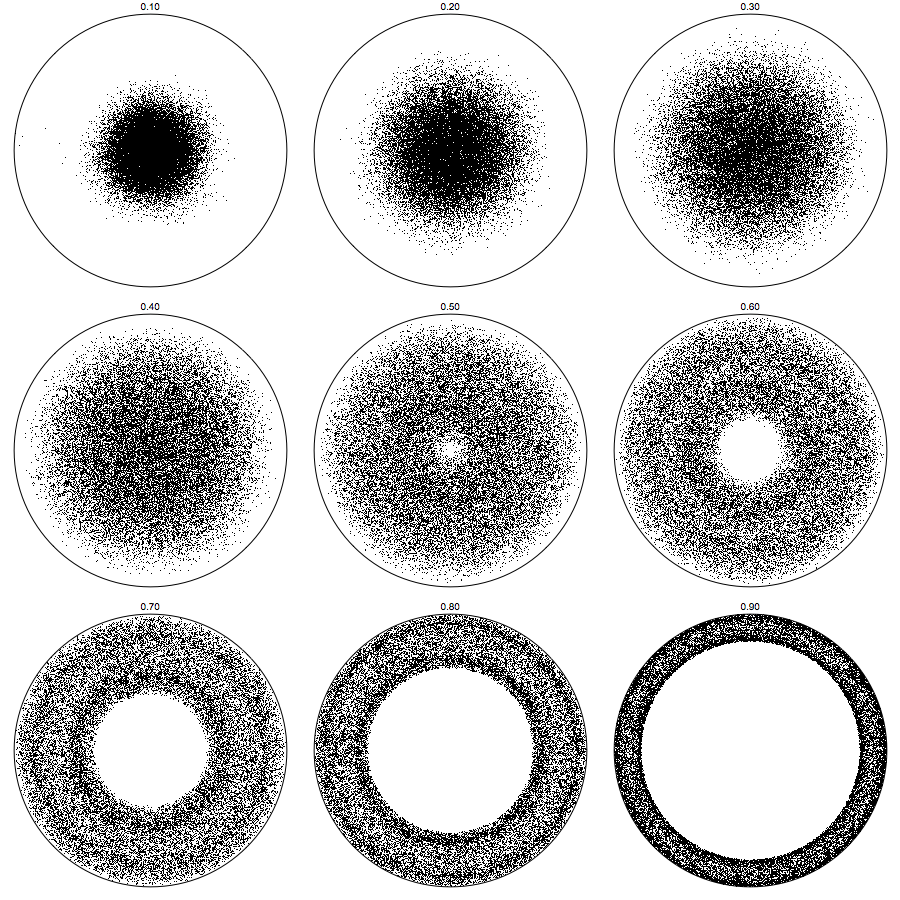
For small alpha it just tends to go the center, and for large alpha we go towards the rim, while the center remains inaccessible.

Probability density function

Let's have a look at PDF of the radial position of the points to see how they are distributed for a range of alpha:

ClearAll[CreateSequence,CreateSequenceHistogram]
CreateSequence[steps_]:=RandomReal[{0,2Pi},steps]
CreateSequenceHistogram[m_,\[Alpha]_,\[Delta]_:0.01]:=Module[{seq,circlepoints,pts,plotdata,colors},
    seq=CreateSequence[m];
    seq=Transpose[{Cos[seq],Sin[seq]}];
    pts=Rest@FoldList[(1-\[Alpha])#1+\[Alpha] #2&,seq];
    Histogram[Norm/@pts,{0,1,\[Delta]},"PDF",Frame->True,PlotLabel->\[Alpha],ImageSize->300,PlotRange->{{0,1},{0,4.5}}]
]
Grid[Partition[CreateSequenceHistogram[10^6,#]&/@Range[0.1,0.8,0.1],UpTo[3]]]

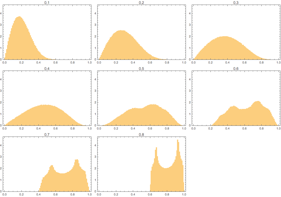
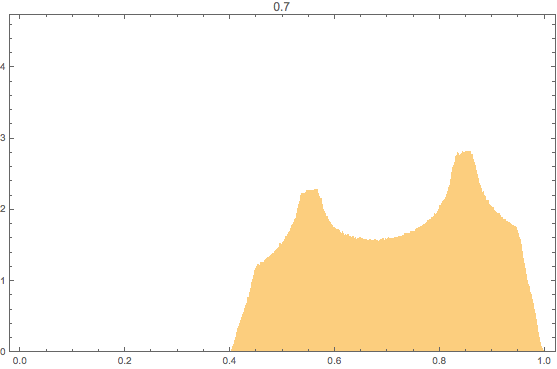
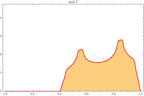
Especially the cases around 0.7 look interesting because of its unexpected shape, let's make high-resolution PDF for that alpha:

CreateSequenceHistogram[10^7, 0.7, 0.001]

So we can calculate this more quickly? Well, let's first look at how a single jump works:

Clear[GetOverView,GetPlot\[Theta]r,GetCDFFunc,GetPDFFunc,r]
GetOverView[b_,\[Alpha]_]:=Graphics[{Circle[],Red,Point[{b,0}],Black,Circle[{(1-\[Alpha])b,0},\[Alpha]]}]
GetPlot\[Theta]r[b_,\[Alpha]_]:=Plot[Sqrt[\[Alpha]^2+(1-\[Alpha])^2 b^2+2\[Alpha] Cos[\[Theta]](1-\[Alpha])b],{\[Theta],0,2Pi},PlotRange->{0,1},AxesLabel->{"\[Theta]","r"},Ticks->{Range[0,2Pi,Pi/2]}]
GetCDFFunc[b_, \[Alpha]_] := \[Piecewise] {
   {0, r < Abs[b (1 - \[Alpha]) - \[Alpha]]},
   {1, r > b (1 - \[Alpha]) + \[Alpha]},
   {((\[Pi] - 
     ArcCos[(b^2 - r^2 - 2 b^2 \[Alpha] + \[Alpha]^2 + 
       b^2 \[Alpha]^2)/(2 b (-\[Alpha] + \[Alpha]^2))])/\[Pi]), \!\(
      TagBox["True",
       "PiecewiseDefault",
       AutoDelete->False,
       DeletionWarning->True]\)}
  }
GetPDFFunc[b_,\[Alpha]_]:=D[GetCDFFunc[b,\[Alpha]],r]
GetPDFFunc[b_, \[Alpha]_] := \[Piecewise] {
   {0, r - Abs[b (1 - \[Alpha]) - \[Alpha]] < 
      0 || -b + r - \[Alpha] + b \[Alpha] > 0},
   {-(r/(b \[Pi] (-\[Alpha] + \[Alpha]^2) Sqrt[
      1 - (b^2 - r^2 - 2 b^2 \[Alpha] + \[Alpha]^2 + 
         b^2 \[Alpha]^2)^2/(
       4 b^2 (-\[Alpha] + \[Alpha]^2)^2)])), \!\(
      TagBox["True",
       "PiecewiseDefault",
       AutoDelete->False,
       DeletionWarning->True]\)}
  }
GetPlotCDF[b_,\[Alpha]_]:=Plot[GetCDFFunc[b,\[Alpha]],{r,0,1},AxesLabel->{"r","CDF(r)"},PlotRangePadding->None]
GetPlotPDF[b_,\[Alpha]_]:=Plot[GetPDFFunc[b,\[Alpha]],{r,0,1},AxesLabel->{"r","PDF(r)"},PlotRangePadding->None]

Manipulate[GraphicsGrid[Partition[{GetOverView[b,\[Alpha]],GetPlot\[Theta]r[b,\[Alpha]],GetPlotCDF[b,\[Alpha]],GetPlotPDF[b,\[Alpha]]},2],Spacings->Scaled[.5],ImageSize->600],{{b,0.78},0,1},{{\[Alpha],0.5},0,1}]

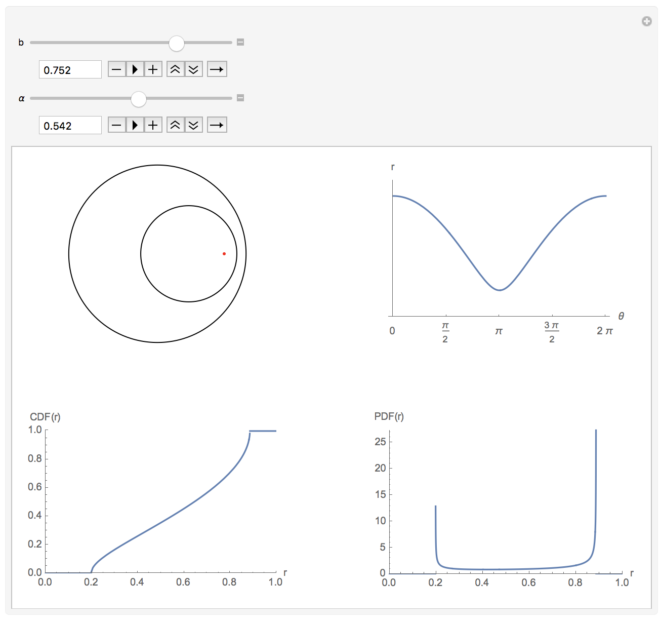
the red point shown above can jump to any position of the inner circle. Top right shows the radius (from the center) as a function of theta for that circle. Bottom left shows the CDF of the possible radial positions, and bottom right the PDF of the possible radial positions. For the shown example you can see it will end up somewhere with a radius between 0.2 and 0.9, and most likely at those edges as the PDF is very large there.

Starting from an initial flat PDF of equal probability as a function of radius we can iterate that PDF to get the next PDF if we 'jump those probabilities':

ClearAll[GetMatrix,DoPDFFind]
GetMatrix[binranges_,\[Alpha]_]:=Module[{midbins,func},
    midbins=MovingAverage[binranges,2];
    Transpose[Table[
        func=GetCDFFunc[Subscript[midbins, [[i]]],\[Alpha]];
        Differences[Table[func,{r,binranges}]]
    ,
        {i,Length[midbins]}
    ]]
]
DoPDFFind[\[Alpha]_,bins_Integer,n_:25]:=Module[{binwidth,initprob,prob,binranges,tmp,mat,plotdata},
    binwidth=1/bins;
    initprob=1/bins;

    prob=N[ConstantArray[initprob,bins]];
    binranges=N[Range[0,1,binwidth]];

    mat=Re[GetMatrix[binranges,\[Alpha]]];

    tmp=bins Nest[mat.#&,prob,n];
    plotdata={MovingAverage[binranges,2],tmp}\[Transpose];
    plotdata=Mean/@Partition[plotdata,2];
    ListLinePlot[plotdata,PlotRange->{{0,1},{0,All}},PlotStyle->Directive[Red,Thick]]
 ]

Now we check if the PDF matches:

\[Alpha]=0.7;
Show[{CreateSequenceHistogram[10^7,\[Alpha],0.001],DoPDFFind[\[Alpha],500]},ImageSize->500,AxesLabel->{"r","PDF(r)"},PlotLabel->Row[{"\[Alpha]=",\[Alpha]}],Frame->True]

We can actually see the convergence:

ClearAll[DoPDFFindAll]
DoPDFFindAll[\[Alpha]_,bins_Integer,n_:25]:=Module[{binwidth,initprob,prob,binranges,tmp,mat},
    binwidth=1/bins;
    initprob=1/bins;

    prob=N[ConstantArray[initprob,bins]];
    binranges=N[Range[0,1,binwidth]];

    mat=GetMatrix[binranges,\[Alpha]];
    mat=Re[mat];

    tmp=bins NestList[mat.#&,prob,n];
    tmp={MovingAverage[binranges,2],#}\[Transpose]&/@tmp;
    tmp=(Mean/@Partition[#,2])&/@tmp;
    ListLinePlot[tmp,PlotRange->{{0,1},{0,All}},Frame->True,PlotLegends->Automatic,ImageSize->600]
]
DoPDFFindAll[0.7,500,5]

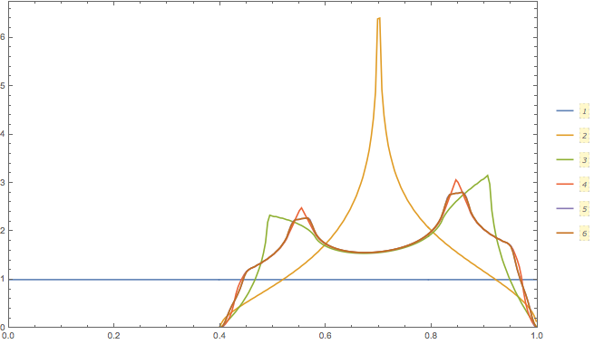
As you can see, it quickly converges to its final form. What we've done here is called a Markov chain, and this entire procedure could've been simplified by using the DiscreteMarkovProcess function in the Wolfram Language:

bins=500;
binwidth=1/bins;
initprob=1/bins;

prob=N[ConstantArray[initprob,bins]];
binranges=N[Range[0,1,binwidth]];
mat=GetMatrix[binranges,0.7];
dmp=DiscreteMarkovProcess[prob,Transpose@mat];
sd=StationaryDistribution[dmp];
sdpdf=PDF[sd,x];
plotdata=Table[{x/bins,bins Chop[sdpdf]},{x,1,bins}];
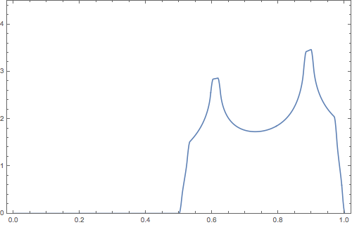
ListPlot[plotdata,Joined->True,Frame->True,ImageSize->500,PlotRange->{0,4.5}]

giving the same result:

That is it for now...