When you magnify a 1-dimensional figure by a factor of 2, you get twice as much. If you have Mathematica (or just a CDF player) you should try the accompanying notebook. When you slide r, the lengths of the blue arc and gold arc remain equal to $ \pi $ , so that together they are $2\pi$. When the r slider = 2, the arcs are quarter circles. (How come nobody says semidemicircles?) But when the r slider reaches 4, both arcs together add up to a quarter circle twice as big:
Manipulate[
 ParametricPlot[{{r Cos[t] + 4 - r,
    r Sin[t]}, {r Cos[\[Pi]/r] + 4 - r,
     r Sin[\[Pi]/r]} + {r Cos[t + 1/8 \[Pi] (r - 2)],
     r Sin[t + 1/8 \[Pi] (r - 2)]} - {r Cos[1/8 \[Pi] (r - 2)],
     r Sin[1/8 \[Pi] (r - 2)]}}, {t, 0, \[Pi]/r}], {r, 2, 4},
 Paneled -> False]
(We allow bending, but not stretching.) So two quarter circles can be joined and bent into one twice as long. If we had 3 quarter circles, we could similarly bend them into a quarter circle three times as long. This idea is even more obvious with line segments (very thin sticks). A long stick broken in half is two sticks half as long.
In 2 dimensions, magnifying a 2 dimensional figure by 2 gives you 4 times as much. Gluing together 4 squares makes a square twice as big. And as we've seen, magnifying a 2 dimensional figure by 3 gives 9 times as much.
In the top two (triangular and square) figures, we also see how magnifying their 1 dimensional boundaries by a factor of 3 gives us three times as much boundary.
But something is screwy with the boundary of that bottom figure. Before we get to it, let's see what happens with magnification in 3 dimensions. A first order Menger Sponge is a cube made of 20 little cubes one third the size:
Graphics3D[Cuboid /@ Select[Tuples[{-1, 0, 1}, 3], #.# > 1 &]]
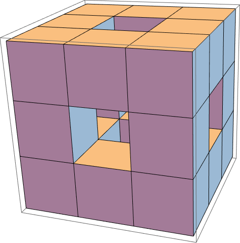
This is $\text{3$\times $3$\times $3 = }3^3\text{= 27}$ cubes minus the one in each face minus the one in the center. But it shows that magnifying a 3 dimensional figure by 3 gives you $\text{3$\times $3$\times $3 = }3^3$ times as much. And you need to glue $\text{2$\times $2$\times $2 = }2^3\text{= 8}$ cubes together to get one magnified by 2. So how much do we get by magnifying a D dimensional figure by a factor of n? $\text{n$\times $n$\times \cdots \times $n (D times)=}n^D\text{(!)}$
Now we can say what is screwy about that tripled boundary. By how much did we magnify? Exactly enough to multiply the enclosed 2 dimensional (D = 2) area by 7. So $n^2= 7$.
Solve[n^2 == 7]
{{n -> -Sqrt[7]}, {n -> Sqrt[7]}}
I'll bet you knew that. The positive answer, anyway. But how can we explain magnifying the boundary by $\sqrt{7}$ and getting 3 copies? The dimension D must be screwy! We have copies = $n^D$. That is, $3 = ((\sqrt{7})^D)$. How in the heck can we solve for D? We need a new function!
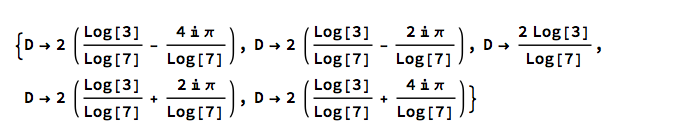
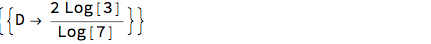
Solve[3 == (Sqrt[7])^D]

Yikes! What's this? It means there are infinitely many possible values of D, one for every integer (whole number) value of the (made up) symbol $C[1]$. Here's a way to try some integers. Make a list of Rules:
Table[{C[1] -> integer}, {integer, -2, 2}]

Then slash-dot applies them (if you have the right number of curly braces):
%%[[1, 1]] /. %
% means the last answer. %% means the one before that. [[1,1]] means the first part of the first part. But this is still confusing. Come on, D is a number. So these things are numbers. What are they, approximately? Gimme 6 digits:
N[%, 6]

What are those little "i"s? It means they're imaginary!
Solve[x*x == -1]

Thank goodness, one of our D values is real--the C[1]->0 (middle) one.
%%%[[3]]

So this is somehow the answer to
3 == (Sqrt[7])^D /. %
True
Convince me harder.
(Sqrt[7])^D /. D -> 1.12915
3.
OK, I'm convinced. (You can type in $\sqrt{7}$ with Control+2 7 rightarrow. (You can type superscript (exponent) D as Control+6 D.) Now let's find a way to solve for D without imaginary answers.
Assuming[D \[Element] Reals, Solve[3 == (Sqrt[7])^D]]

Doesn't work. We need something better than Solve. Its name is Reduce.
Reduce[3 == (Sqrt[7])^D, D, Reals]

Ahhh. But wait, Solve works here too!
Solve[3 == (Sqrt[7])^D, D \[Element] Reals]
D $\in$ Reals means D is real. It's the same as
Element[D, Reals]

You can type $\in$ as esc el esc.
So now we know how to solve $a = b^x$ for x. Or do we?
Solve[a == b^x, x \[Element] Reals]

We need something called Refine.
Refine[Solve[a == b^x, x], x \[Element] Reals]
We pronounce this "log of a to the base b", more briefly it can be typed in as
Log[b, a]

Mathematicians usually write this with subscripts:
Log[b, a] == Subscript[Log, b][a] == Subscript[Log, b]@a ==
  Subscript[Log, b]@a // Simplify

But if Mathematica recognized this as an equality, it would have reduced it to True. We have
E^Log[x] == x
True
What about
Log[E^x] == x

Why didn't that reduce to True?
Assuming[x \[Element] Reals, FullSimplify@%]
True
So something bad probably happens when x is imaginary. Try
%% /. x -> I
True
It failed to fail! We can look for a place where it does.
FindInstance[Log[E^x] != x, x]

Log[E^x] /. %

log(exp()) added $2 I \pi $ (!). Let's plot |error| over an $100 \times 100$ neighborhood of 0+0i
Log[E^z] - z /. z -> x + I y

Plot3D[Abs@%, {x, -50, 50}, {y, -50, 50}, PlotPoints -> 50,
 AxesLabel -> Automatic]
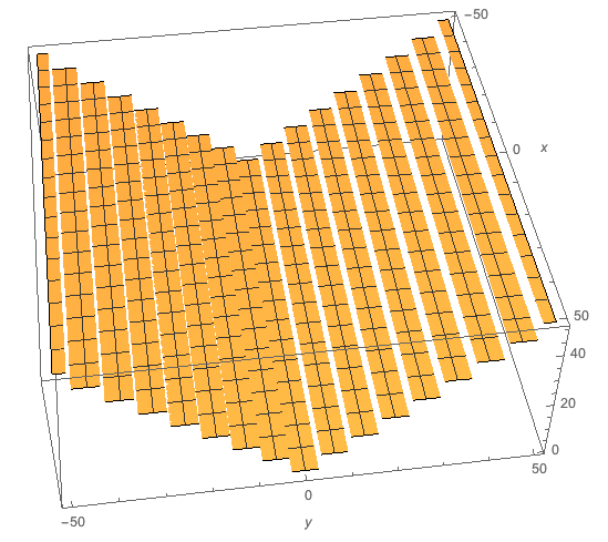
Bleachers! So all the errors must be a multiples of i $\pi$. And not care about x.
Plot[(Log[E^(I y)] - I y)/I/\[Pi], {y, -50, 50}]
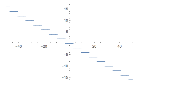
Plot[Log[E^(I y)]/I/\[Pi], {y, -9, 9}]
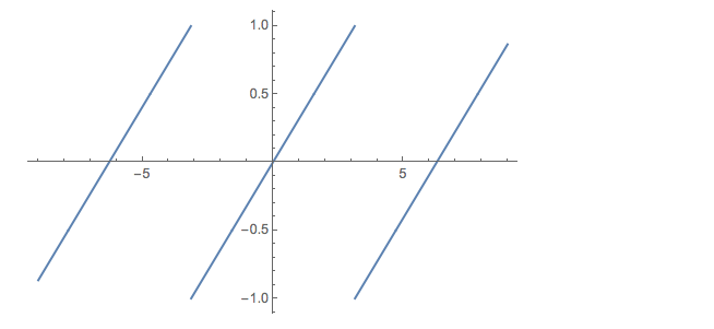
This resembles
Plot[Mod[x/\[Pi], 2], {x, -9, 9}]
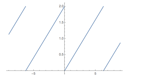
except advanced half a period and lowered half an amplitude. Mathematica's Mod function takes an optional third argument that does just what we need:
Plot[Mod[x/\[Pi], 2, -1], {x, -9, 9}]
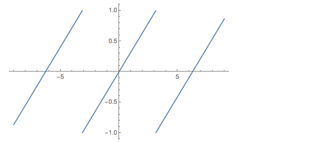
Simple but important: At least for real numbers,
# == Distribute[#, Mod] &[a Mod[x, m, y]]

Assuming[a > x > m > y > 0, FullSimplify@%]

FullSimplify doesn't (yet) know this. But
FindInstance[! %, {a, x, m, y}, Reals]
{}
FindInstance flatly says there are none. So it seems that
Log[E^(x + I y)] == x + I Mod[y, 2 \[Pi], -\[Pi]]

But why didn't it say True? Well it probably isn't unless x and y are real:
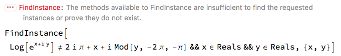
FindInstance[
 Not@% && x \[Element] Reals && y \[Element] Reals, {x, y}]
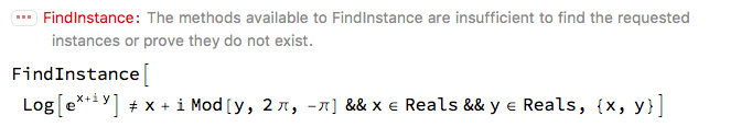
So it might be true. Can Mathematica prove it automatically?
FullSimplify[%%, x \[Element] Reals && y \[Element] Reals]

No, probably because it's not true! Adam Strzebonski of Wolfram Research reports a counterexample: x=0, y=$\pi$ yields the absurdity - i $\pi$= i $\pi$. Why didn't we see this with the "bleachers" plot? Because the error is only one point thick along the edge of each bench. It's like the difference between $\text{$\lfloor $y$\rfloor $ vs $\lceil $y$\rceil $ - 1}$ (floor(y) vs ceiling(y)-1).
The corrected formula is slightly uglier:
Log[E^(x + I y)] == x + 2 I \[Pi] + I Mod[y, -2 \[Pi], -\[Pi]];
FullSimplify[%, x \[Element] Reals && y \[Element] Reals]

Sadly, this should say True. But sometimes, seeking a counterexample with FindInstance will elicit the claim that there are none.
FindInstance[! % && x \[Element] Reals && y \[Element] Reals, {x, y}]
Sadly, it's not smart enough to prove there are none. (Notice that Mathematica's prefix ! means Not, not Factorial or the like. And notice that it changed = to !=.)
We should mention that Mod's third argument, if present, is initially subtracted from the first, and then added to the result. This is an example of the ubiquitous construct prepare $\circ$ doit $\circ$ cleanup, where cleanup undoes the prepare. In symbols $f^{-1}\circ g \circ f$. Mathematicians describe this with the overused word conjugation, but we could call it footscratching: Itch? remove-shoe $\circ$ scratch-foot $\circ$ replace-shoe. Or open-drawer $\circ$ grab-Desenex $\circ$ close-drawer.
What is the number whose Log is 1?
Solve[Log[b] == 1]

This is the famous "base of natural logarithms", typed as capital E:
Log@E
1
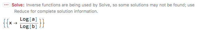
Reduce[a == E^x, x, Reals]
![enter image description here][35]
This says a must be positive for its log to be real. Believe it or not, you are already familiar with imaginary logarithms of negative numbers. Surely you've heard
E^(I \[Pi])
-1
This makes $\pi$ the logarithm of -1 to the base $e^i$ (!)
Log[E^I, -1]
$\pi$
Further evidence that $\pi$ is a logarithm: What is the formula for this sequence?
{1, -1/2, 1/3, -1/4, 1/5, -1/6}

FindSequenceFunction[%, n]

I.e,
Table[%, {n, 6}]

Here are two different ways to add these up:
{Total@%, Sum[%%, {n, 6}]}

But with Sum, we needn't stop with 6, or anywhere else! What is the infinite sum?
Sum[%%%, {n, \[Infinity]}]
Log[2]
( $\infty$ is option 5.) Suppose instead we sum the alternating reciprocal odd numbers.
Table[(-1)^n/(1 - 2 n), {n, 6}]

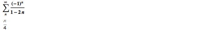
(This was typed as Sum[( $(-1)^n$)(1-2n),{n,$\infty$}] later followed by control shift t.) Replacing $(-1)^n$ by $x^n$, (minus) this is a special case of
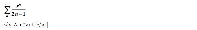
(It's minus because we changed 1-2n to 2n-1.) But what's ArcTanh??
Factor@TrigToExp@%

It's made of logarithms! And the two logarithms combine into one!
Assuming[x \[Element] Reals, MapAt[Log@FullSimplify@Exp@# &, %, 3]]

Undoing that we replaced $(-1)^n$ by $x^n$,
% /. x -> -1
-$\pi$/4
But wait a minute, that part where we turn ArcTanh into Log is hard to understand. One easy important thing is that the function that raises e to the power x, i.e., $e^x$ is so important that people named it Exp(x):
Exp@x == Exp[x] == E^x
True
Another fairly easy very important thing: If we divide the true equation
x == a^Log[a, x]
True
by the true equation
y == a^Log[a, y]
True
we get
x/y == a^(Log[a, x] - Log[a, y])
True
But obviously
x/y == a^Log[a, x/y]
True
so, equating the exponents,
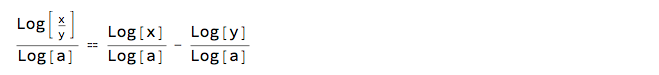
Log[a, x/y] == Log[a, x] - Log[a, y]
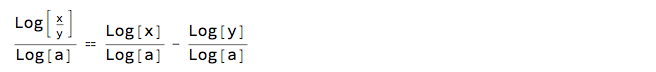
The log of the quotient is the difference of the logs! Usually. But here's why Mathematica didn't wise off as usual and reduce this to True:
% /. {x -> E, y -> -E} // Expand

Let's just look at a = e (natural logs) and real x, y and see where
Subtract @@ %% /. a -> E

differs from 0.
Plot3D[Abs[%], {x, -2, 2}, {y, -2, 2}, AxesLabel -> Automatic]
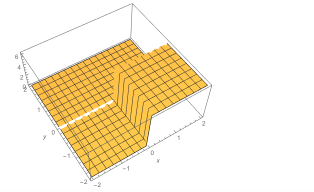
So we need to avoid the quadrant x>=0, y<=0. What is Log[0], by the way? I.e., to what power must we raise e to get 0?
Log[0]
-$\infty$
Returning to ArcTanh, we can now use our log(quotient) rule
-(1/2) Sqrt[x] (Log[1 - Sqrt[x]] - Log[1 + Sqrt[x]]) /.
 Log@a_ - Log@b_ :> Log[a/b]

% /. x -> -1
-$\pi$/4
But we didn't have that rule, so I wanted Mathematica to simplify it automatically. Unfortunately, Mathematica is too clever:
FullSimplify[-(1/2) Sqrt[x] (Log[1 - Sqrt[x]] - Log[1 + Sqrt[x]])]

What about just
FullSimplify[Log[1 - Sqrt[x]] - Log[1 + Sqrt[x]]]

Still too clever! Trick: Take Exp, simplify, then take log:
FullSimplify[Exp[Log[1 - Sqrt[x]] - Log[1 + Sqrt[x]]]] // Log

foo//f is the same as f@foo is the same as f[foo]. Look up MapAt under Help[Wolfram Documentation]. We didn't use the quotient rule here, so it's probably trustworthy for all real and complex (= mixed real and imaginary) x.
So, if the log of a quotient is the difference of the logs, what is the log of a product? Fairly obviously, the sum of the logs. Which you can figure out from the quotient rule, and the very important rule for log of a power. Just raise
x == a^Log[a, x]
to the p power:
x^p == (a^Log[a, x])^p == a^(p Log[a, x])
True
x^p == (E^Log[x])^p == E^(p Log[x])
True
and then take the log:
Log[x^p] -> Log[(E^Log[x])^p] -> Log[E^(p Log[x])]

Bleep. Outsmarted again. The only way I have found to prevent this is to deliberately mistype p Log[x] as pLog[x], where pLog is any undefined function. Then
Assuming[pLog[x] \[Element] Reals,
 Log[x^p] -> Log[(E^Log[x])^p] -> Simplify[Log[E^pLog[x]]]]

Then finally confess
% /. pLog[x] -> p Log@x

At long last, the log of the $p^{th}$ power of something is p times its log. An important special case is p = -1, the reciprocal function:
% /. p -> -1

The log of something's reciprocal is the negative of its log. Then we can use the quotient rule
Log[x/y]/Log[a] == Log[x]/Log[a] - Log[y]/Log[a]
or just
% /. a -> E

with
% /. y -> 1/z

But
Log[1/x_] -> -Log[x];
(x_ is a pattern) so
%% /. %
Log[x z] == Log[x] + Log[z]
as long ago promised.
An interesting relation between the reciprocal function 1/x and log(x): Plotting y = 1/x makes a hyperbola (blue curve). The area under that hyperbola between 1 and x is log(x) (gold curve):
Manipulate[
 Show[Plot[#, {t, 0, 9}, AspectRatio -> Automatic,
     PlotRange -> {{0, 9}, {-3, 3}}],
    Plot[{#, Evaluate[Integrate[#, t]]}, {t, 1, x},
     Filling -> {1 -> {Axis, Green}}]] &[1/t],
 Item["log x" == Dynamic[Log@x]], {x, 0, 9}]
(Area to the left of x=1 counts negative.) Notice our previous results Log(0) = -$\infty$, Log(1) = 0. Click the square $\oplus$. To see log(1/2), slide the green to the 1st tick, putting .5 in the readout. Or type .5 into it. Now slide to x=2.
Lastly(?!), you've probably heard that
anything^0 == 1
True
(although this is arguable when anything = 0). Now consider the quantity
(anything^p - 1)/p
for small values of p and a few values of anything, say 1/$\pi$, 1/3, 1/e, 1/2, 1, 2, e, 3, and $\pi$:
Table[(anything^p - 1)/p, {anything, {1/\[Pi], 1/3, 1/E, 1/2, 1, 2,
   E, 3, \[Pi]}}]

Plot them all for -1<p<1:
Plot[%, {p, -1, 1}]
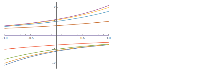
Notice that the values are vertically symmetric about 0 in the middle, where p=0. Let's look there.
%% /. p -> 0
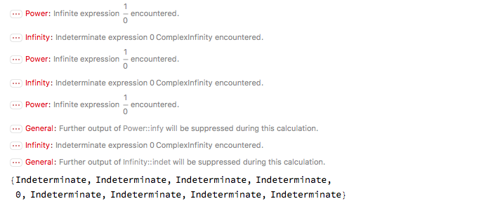
Shame on us!--we divided by 0. But Indeterminate is not what we usually get when we
1/0

We actually did
(1 - 1)/0 == 0/0
(Notice it didn't say True!) But the graph doesn't show any gap at p=0. It shows the curves smoothly crossing the vertical axis in nine places. What are those places? To avoid 0/0, we can instead ask what happens when p becomes infinitely small:
Limit[{(-1 + \[Pi]^-p)/p, (-1 + 3^-p)/p, (-1 + E^-p)/p, (-1 + 2^-p)/p,
   0, (-1 + 2^p)/p, (-1 + E^p)/p, (-1 + 3^p)/p, (-1 + \[Pi]^p)/p},
 p -> 0]

Logarithms! Note that those on the left are the negatives of those on the right, because, for the numbers whose logs we took, those on the left were the reciprocals of those on the right. And the one in the middle was the reciprocal of itself! So its log is the negative of itself!


