One of the well-known algorithm of doing the inverse square root:
$$\frac{1}{\sqrt{x}}$$
is the so-called "fast inverse square root" algorithm, see wikipedia. This code gives a very good approximation of this function, possibly good enough for lighting in video-games. Even now, with modern CPUs, with many new instructions, this is still quite a bit faster than the actual inverse square root. The most surprising thing about this code is the appearance of a magic constant (note that this is C code, including the original comments)
float Q_rsqrt( float number )
{
    long i;
    float x2, y;
    const float threehalfs = 1.5F;

    x2 = number * 0.5F;
    y  = number;
    i  = * ( long * ) &y;                       // evil floating point bit level hacking
    i  = 0x5f3759df - ( i >> 1 );               // what the f*ck?
    y  = * ( float * ) &i;
    y  = y * ( threehalfs - ( x2 * y * y ) );   // 1st iteration

    return y;
}
As you can see, the input is a float (a 32 bit floating point number), which is cast in to a long integer, the bits are shifted, and the result subtracted from a magic constant, this number is then re-interpreted again as a float.
To understand why this works is actually quite a long story, but realise that floats are stored as 32 bits as follows:
SEEEEEEEEMMMMMMMMMMMMMMMMMMMMMMM
where S= sign, E = exponent, and M = Mantissa. So once you interpret this as a long, and start shifted bits, you can get very unpredictable behavior. The question that I'm after is: can this constant be improved?
Let's create a library function in c and link it back in to Mathematica, such that we can try different magic constants and different values x:
Needs["CCompilerDriver`"]
src="
#include \"WolframLibrary.h\"
DLLEXPORT mint WolframLibrary_getVersion(){
  return WolframLibraryVersion;
}
DLLEXPORT int WolframLibrary_initialize( WolframLibraryData libData) {return 0;}
DLLEXPORT void WolframLibrary_uninitialize( WolframLibraryData libData) {return;}
DLLEXPORT int constantzero(WolframLibraryData libData, mint Argc, MArgument *Args, MArgument Res){
   MArgument_setInteger(Res, 0);
   return LIBRARY_NO_ERROR;
}
DLLEXPORT int fastinvsqrt(WolframLibraryData libData, mint Argc, MArgument *Args, MArgument Res) {
    double in = MArgument_getReal(Args[0]);
    int magic = MArgument_getInteger(Args[1]);
    float x = in;
    float halfx = 0.5f * x;
    int i = *(int*)&x;
    i = magic - (i >> 1);
    x = *(float*)&i;
    x = x*(1.5f-(halfx*x*x));
    double I1;
    I1 = x;
    MArgument_setReal(Res, I1);
    return LIBRARY_NO_ERROR;
}";
Quiet@LibraryFunctionUnload[fastinvsqrt]
fastinvsqrtlib=CreateLibrary[src,"fastinvsqrt"]
fastinvsqrt=LibraryFunctionLoad[fastinvsqrtlib, "fastinvsqrt",{Real,Integer},Real]
magicconst=16^^5f3759df
Plot[{1/Sqrt[x],fastinvsqrt[x,magicconst]},{x,0.1,5},PlotRange->{0,2}]
LogLogPlot[{1/Sqrt[x]-fastinvsqrt[x,magicconst],1/Sqrt[x]},{x,0.01,100000},PlotRange->{All,{10^-6,10}},Frame->True,PlotRangePadding->None,PlotPoints->1200,MaxRecursion->3]
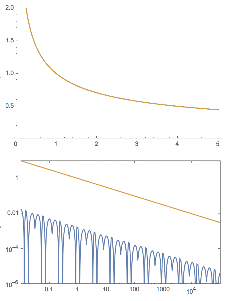
The match is indeed great! and we can see that the error (second plot, in blue) is of the order 0.1% of the result for the original magic constant!
Let's introduce the relative error:
ClearAll[relativeerror]
relativeerror[x_Real, magic_Integer] := (1/Sqrt[x] - fastinvsqrt[x, magic])/(1/Sqrt[x])
and plot it:
LogLogPlot[relativeerror[x, magicconst], {x, 0.01, 100000},
 Frame -> True, PlotRangePadding -> None, PlotRange -> {10^-5, 1},
 PlotPoints -> 1200, MaxRecursion -> 3]
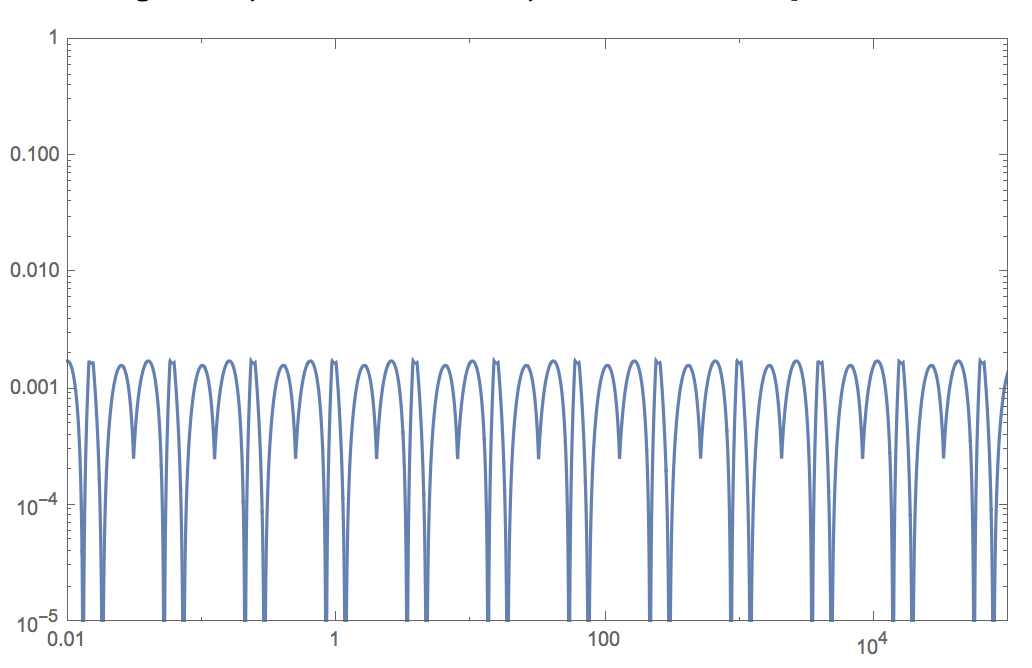
This plot is periodic because of the way floating point numbers are defined/implemented, we can zoom in on one of the parts:
LogLinearPlot[relativeerror[x, magicconst], {x, 1, 4}, Frame -> True,
 PlotRangePadding -> None, PlotRange -> All, PlotPoints -> 1200,
 MaxRecursion -> 3]
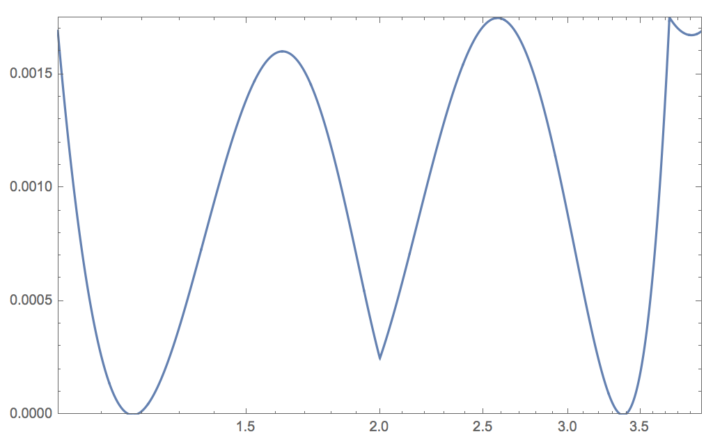
We can plot slight deviations from the magic constant to see the new relative errors:
LogLinearPlot[{relativeerror[x, magicconst],
  relativeerror[x, magicconst - 20000],
  relativeerror[x, magicconst + 20000]}, {x, 1, 4}, Frame -> True,
 PlotRangePadding -> None, PlotRange -> All, PlotPoints -> 1200,
 MaxRecursion -> 3, PlotLegends -> {"0", "-20000", "+20000"}]
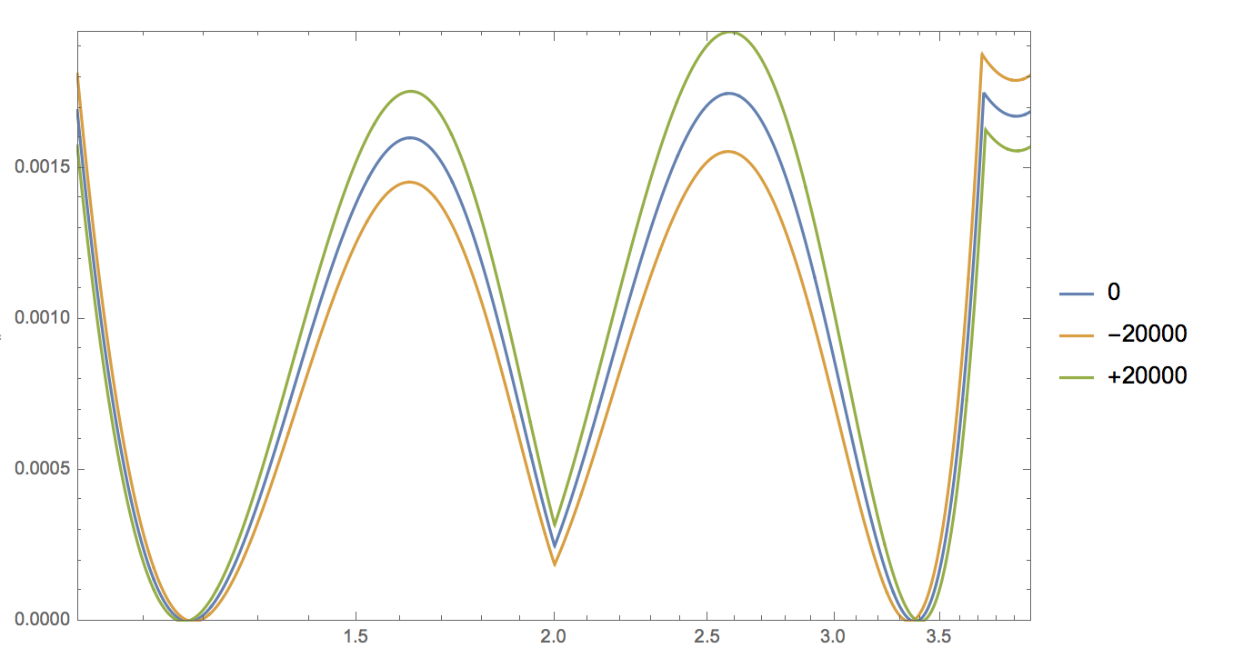
If the constant increases, the center peaks go up, but the far-right and far-left peak go down.
Let's try a bunch of magic-constants, and check the maximum (relative) error we find. I do this by sampling many point and looking for the maximum error I find in those points:
Dynamic[d]
data = Table[{d,  Max[Table[With[{x = 2^s}, ((1/Sqrt[x] - fastinvsqrt[x, d + magicconst])/(1/Sqrt[x]))], {s, 0, 2, 0.00001}]]}, {d, -100000, 100000,
    1000}];
data // ListLogPlot
TakeSmallestBy[data, Last, 1]
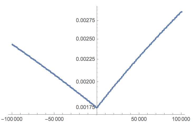
{{0, 0.00175225}}
If there is a better constant, it sure is close to the original constant. Let's zoom in a bit:
Dynamic[d]
data = Table[{d,  Max[Table[With[{x = 2^s}, ((1/Sqrt[x] - fastinvsqrt[x, d + magicconst])/(1/Sqrt[x]))], {s, 0, 2, 0.00001}]]}, {d, -1000, 1000, 10}];
data // ListLogPlot
TakeSmallestBy[data, Last, 1]
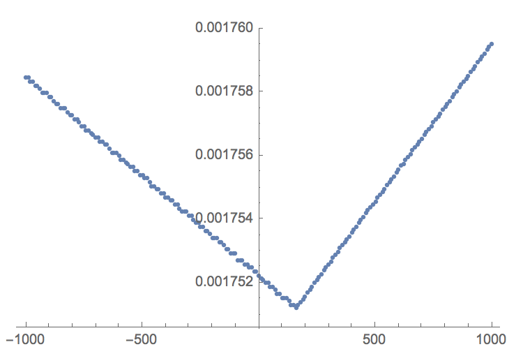
{{160, 0.00175121}}
We can zoom in even further:
Dynamic[d]
data=Table[{d,Max[Table[With[{x=2^s},((1/Sqrt[x]-fastinvsqrt[x,d+magicconst])/(1/Sqrt[x]))],{s,0,2,0.0000001}]]},{d,160,170,1}];
data//ListLogPlot
TakeSmallestBy[data,Last,1]
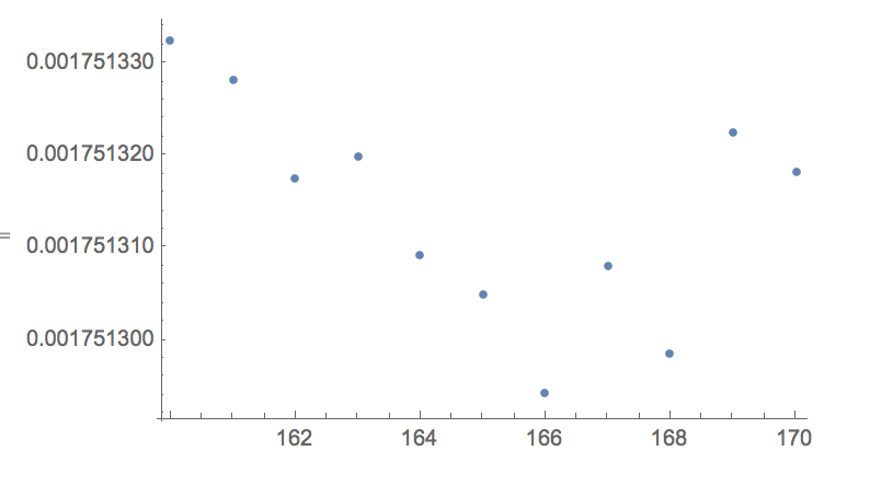
{{166, 0.00175129}}
magicconstant + 166 seems to have a slightly better worst-case performance. This corresponds to the follow new magic constant:
BaseForm[magicconst + 166, 16]
or in C (in hex):
0x5f375a85
We could also use the built-in FindMaximum:
ClearAll[FindMaxima]
FindMaxima[d_Integer]:=Module[{x},
    Max[Table[First@FindMaximum[((1/Sqrt[x]-fastinvsqrt[x,d+magicconst])/(1/Sqrt[x])),{x,x0,1,4},MaxIterations->5000,WorkingPrecision->50],{x0,1.0,4.0,0.03}]]
]
Now using this function and look around our probable minimum:
Dynamic[d]
data=Quiet@Table[{d,FindMaxima[d]},{d,150,175,1}];
data//ListLogPlot
TakeSmallestBy[data,Last,1]
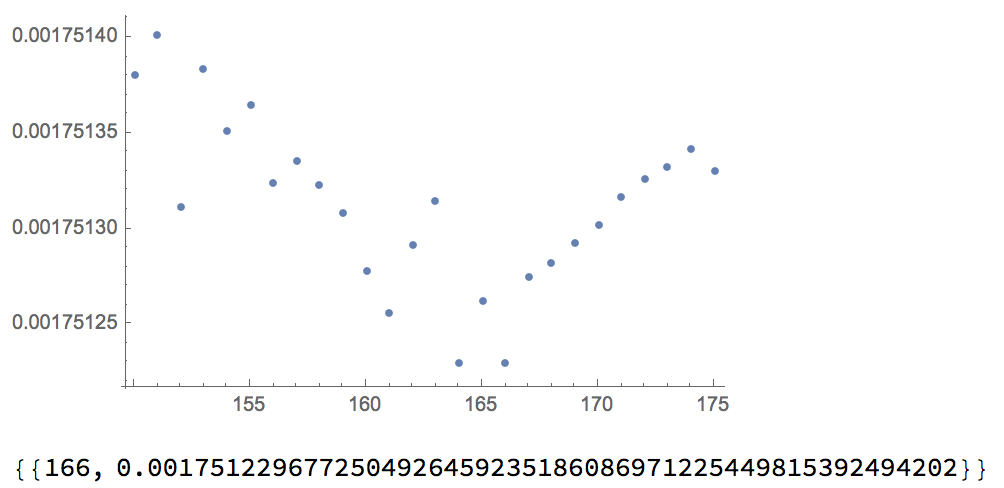
Which also find 166. So that seems to be in agreement. Another paper found 0x5f375a86 which 16^^5f375a86 - magicconst = 167. So perhaps he/me is wrong with rounding somehow
Average error
So far, we've been looking at maximum error possible, but what about minimising the average error? Since we're using floating point numbers that can range over many many decades I would like to minimize the following integral of the error:
Integrate[relativeerror[2^s]^2,{s,0,2}]
Note that I do not sample the domain x 1 to 4 linearly. Again we can run for large deviations from the magic constant:
Dynamic[d]
data=Table[{d,Total[Table[With[{x=2^s},((1/Sqrt[x]-fastinvsqrt[x,d+magicconst])/(1/Sqrt[x]))^2],{s,0,2,0.00001}]]},{d,-250000,250000,10000}];
data//ListLogPlot
TakeSmallestBy[data,Last,1]
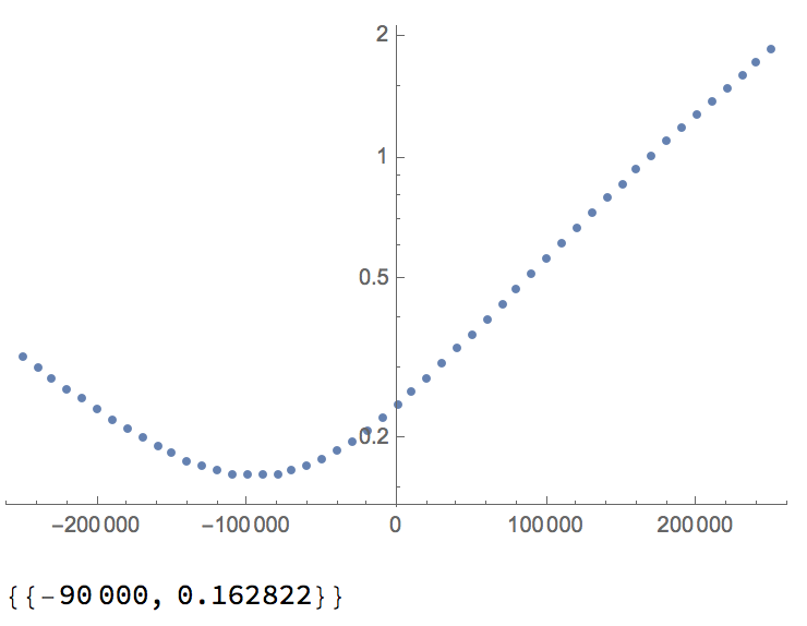
Let's zoom in a bit more:
Dynamic[d]
data=Table[{d,Total[Table[With[{x=2^s},((1/Sqrt[x]-fastinvsqrt[x,d+magicconst])/(1/Sqrt[x]))^2],{s,0,2,0.00001}]]},{d,-96000,-94000,20}];
data//ListLogPlot
TakeSmallestBy[data,Last,1]
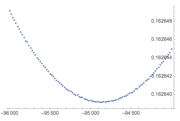
And zooming a bit more and using a smaller 'integration' steps:
Dynamic[d]
data=Table[{d,Total[Table[With[{x=2^s},((1/Sqrt[x]-fastinvsqrt[x,d+magicconst])/(1/Sqrt[x]))^2],{s,0,2,0.00000005}]]},{d,-94900,-94800,1}];
data[[All,2]]=Rescale[data[[All,2]]];
ListPlot[data,PlotRange->All]
TakeSmallestBy[data,Last,1]
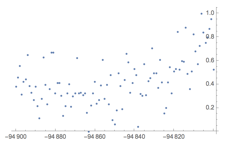
The lowest value happens at magicconstant - 94863:
LogLogPlot[{relativeerror[x,magicconst],relativeerror[x,magicconst-94863]},{x,0.01,100000},Frame->True,PlotRangePadding->None,PlotRange->{10^-5,1},PlotPoints->1200,MaxRecursion->3]
LogLinearPlot[{relativeerror[x,magicconst]^2,relativeerror[x,magicconst-94863]^2},{x,1,4},Frame->True,PlotRangePadding->None,PlotRange->All,PlotPoints->1200,MaxRecursion->3]
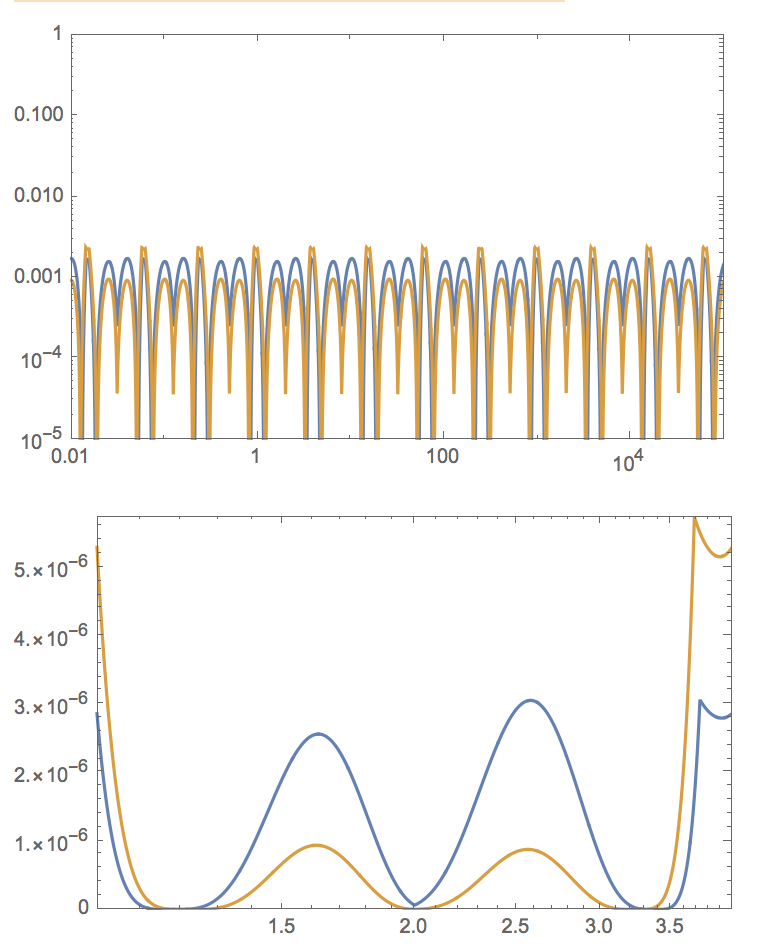
Here (in orange) the average (square) relative error is better as compared to the original constant.
Hope you enjoyed this little exploration of using C code inside Mathematica and to optimize low-level algorithms interactively using Mathematica's library functionality and plotting functionality. The original code includes a single Newton iteration to further hone in to the correct answer, the plots I've showed are for a single iteration. Other people have optimized the constant for not a single iteration or two iterations
So there are different constants out there. And, since the values are always under-estimated, the Newton iteration can also be modified to account for this.