Predicting the properties of a chemical can be difficult and costly. Experiments are time consuming and expensive, and quantum mechanical simulations require a lot of computing time. It would be highly advantageous to predict properties from the structure alone. This method is known as QSPR or QSAR, and it is widely used in the pharmaceutical industry to predict properties of drugs. Here I will present a machine learning approach to QSAR.
ChemicalData[] contains roughly 44,000 chemicals with a large amount of associated data. Given the sophisticated machine learning and neural network functions in Mathematica, it should be plausible to predict some of the data based on the structure. I selected chemicals containing nothing except Carbon, Hydrogen, Oxygen, and Nitrogen to get a simple subset of organic molecules. I removed compounds with insufficient data and compounds with non-standard isotopes. This created a subset of about 5500 chemicals. The properties predicted are melting point, boiling point, heat of vaporization, heat of fusion, and heat of combustion.
The code used here can be found at GitHub:
https://github.com/MarcThomson/WSS2017_Project
Downloading Data
First, define the properties to get from the database.
 molecularProperties = {"SMILES",
                  "BondCounts",
                  "VaporizationHeat",
                  "CombustionHeat",
                  "FusionHeat",
                  "FormalCharges",
                  "NetCharge",
                  "PartitionCoefficient",
                  "TopologicalPolarSurfaceArea",
                  "NonStandardIsotopeNumbers",
                  "AtomPositions",
                  "VertexTypes",
                  "BoilingPoint",
                  "MeltingPoint",
                  "MolarMass",
                  "AdjacencyMatrix",
                  "RotatableBondCount",
                  "HBondAcceptorCount",
                  "HBondDonorCount",
                  "BlackStructureDiagram",
                  "Name"};
Once this is done, the data can be downloaded and formatted into an association of associations. The format is name->{property->value}
totalSetRaw =
   RandomSample[ChemicalData[], molecularProperties]; // Timing

propertiesExceptName = molecularProperties[[1 ;; -2]];
names = totalSetRaw[[;; , -1]];
totalSetBase = Association[Map[#1 -> propertiesExceptName &, names]];
totalSet =
  Association[
   Table[names[[i]] ->
     Association[
      Thread[totalSetBase[[names[[i]]]] ->
        totalSetRaw[[i, ;; -2]]]], {i, 1, Length[totalSetRaw]}]];
Finally, the set is filtered to make sure the chemicals satisfy the criteria.
 requiredProperties[A_] := And[Not[MissingQ[A["SMILES"]]],
                     StringQ[A["SMILES"]],

                     Not[MissingQ[A["AdjacencyMatrix"]]],
                     ArrayQ[A["AdjacencyMatrix"]],
                     Total[Total[A["AdjacencyMatrix"]]] > 0,

                     Not[MissingQ[A["BoilingPoint"]]],
                     QuantityQ[A["BoilingPoint"]],

                     Not[MissingQ[A["MolarMass"]]],
                     QuantityQ[A["MolarMass"]],

                     Not[MissingQ[A["MeltingPoint"]]],
                     QuantityQ[A["MeltingPoint"]],

                     Not[MissingQ[A["AtomPositions"]]],
                     ListQ[A["AtomPositions"]],

                     Not[MissingQ[A["HBondDonorCount"]]],
                     IntegerQ[A["HBondDonorCount"]],

                     Not[MissingQ[A["HBondAcceptorCount"]]],
                     IntegerQ[A["HBondAcceptorCount"]],

                     Not[MissingQ[A["RotatableBondCount"]]],
                     IntegerQ[A["RotatableBondCount"]],

                     Not[MissingQ[A["TopologicalPolarSurfaceArea"]]],
                     QuantityQ[A["TopologicalPolarSurfaceArea"]],

                     Not[MissingQ[A["PartitionCoefficient"]]],
                     NumberQ[A["PartitionCoefficient"]],

                     Not[MissingQ[A["NetCharge"]]],
                     NumberQ[A["NetCharge"]],

                     Not[MissingQ[A["FormalCharges"]]],
                     ListQ[A["FormalCharges"]],

                     Not[MissingQ[A["BondCounts"]]],

                     Not[MissingQ[A["VertexTypes"]]],
                     SubsetQ[{"C", "O", "H", "N"},
    DeleteDuplicates[A["VertexTypes"]]],
                     Length[DeleteDuplicates[A["VertexTypes"]]] > 1,
                     SubsetQ[A["VertexTypes"], {"C"}],

                     Not[MissingQ[A["NonStandardIsotopeNumbers"]]],
                     And @@
    Map[Not[IntegerQ[#]] &, A["NonStandardIsotopeNumbers"]]]


 totalSet = Select[totalSet, requiredProperties[#] &];
At this point, it is useful to save this set. Downloading this data can take many hours, so it is best to do it only once.
Feature Extraction
The heart of this project is selecting the proper features from each molecule.
Subgraphs
The first class of features is the subgraphs, which roughly correlates to functional groups. Molecular properties are generally dependent on these functional groups. Rather than look for functional groups directly, I chose to look for unique subgraphs of the molecule. Unique subgraphs have the same non-Hydrogen atoms and all their attached Hydrogens.
The required code is:
graphSize = {1, 2, 3, 4};

heavyVertices[g_, vertexTypes_] :=
 Select[VertexList[g], vertexTypes[[#]] != "H" &]
lightVertices[g_, vertexTypes_] :=
 Select[VertexList[g], vertexTypes[[#]] == "H" &]

bondsBetween[i_, j_, g_] := 0 /; Equal[i, j]
bondsBetween[i_, j_, g_] := With[{vList = VertexList[g]},
                     Length[
                     Cases[
                       EdgeList[g], vList[[i]] <-> vList[[j]]
                          ]
                         ] +
                       Length[
                     Cases[
                       EdgeList[g], vList[[j]] <-> vList[[i]]
                          ]
                         ]
                     ] /; Not[Equal[i, j]]


subgraphList[graph_, graphSize_, vertexTypes_] := Distribute[
                                 NeighborhoodGraph[
                                  graph,
                                  heavyVertices[graph, vertexTypes],
                                  graphSize
                                  ],
                                 List];

hydrogenSubgraphList[graph_, graphSize_, vertexTypes_] :=
                                   Map[
                                      Subgraph[
                                        graph,
                                        ConnectedComponents[
                                          Subgraph[
                                             graph,
                                             {VertexList[#],
         lightVertices[graph, vertexTypes]}
                                             ]
                                          ][[1]]] &,
                                      subgraphList[graph, graphSize, vertexTypes]];

canonicalAdjM[g_, vertexTypes_] := {
                      With[{
                            sortedList = SortBy[
                                    Range[Length[VertexList[g]]],
                                    -KatzCentrality[g, 0.1][[#]] &]},
                        Table[
                               bondsBetween[i, j, g],
                               {i, sortedList},
                               {j, sortedList}]],
                      With[{
                            sortedList = SortBy[
                                    Range[Length[VertexList[g]]],
                                    -KatzCentrality[g, 0.1][[#]] &]},
                        vertexTypes[[
                               VertexList[g][[sortedList]]
                               ]]
                        ]
                      }

subAdjMList[graph_, graphSize_, vertexTypes_] := Map[
                                canonicalAdjM[
                                      Subgraph[graph, #],
                                      vertexTypes] &,
                                DeleteDuplicatesBy[
                                  hydrogenSubgraphList[graph, graphSize, vertexTypes],
                                  {
                                      {Sort[heavyVertices[#, vertexTypes]]},
                                      Length[lightVertices[#, vertexTypes]]
                                   } &
                                 ]
                                ]
For example, take the molecule 2-Hydroxy-4-Methoxybenzoic Acid.
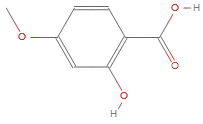
g = AdjacencyGraph[
    ChemicalData["2Hydroxy4MethoxybenzoicAcid", "AdjacencyMatrix"]];
 vl = ChemicalData["2Hydroxy4MethoxybenzoicAcid", "VertexTypes"];
 Graph[AdjacencyGraph[#[[1]]],
    VertexLabels -> Thread[Range[Length[#[[2]]]] -> #[[2]]]] & /@
  subAdjMList[g, graphSize, vl]
The unique substructures are found to be: 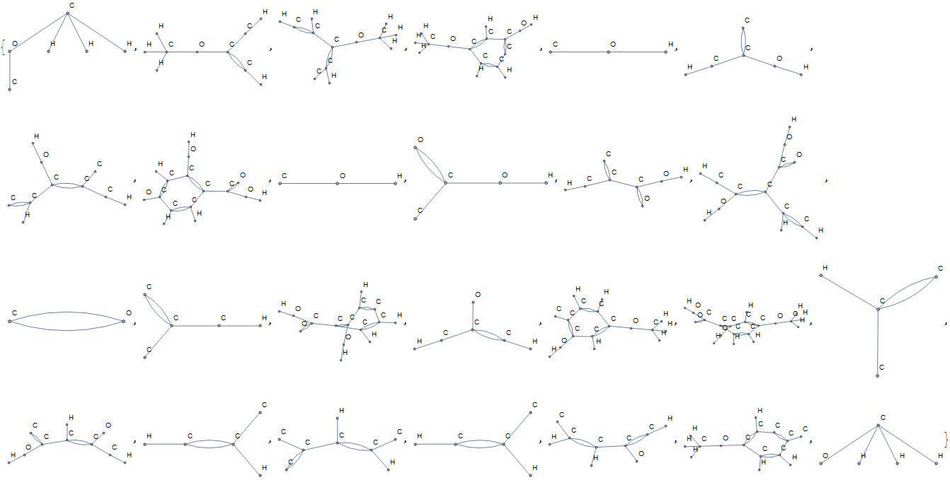
Some of these structures are carboxylic acids, alcohols, and ethers, whereas many others are unnamed.
These features must be turned into numeric values for the machine learning algorithm. To do so, the subgraphs are turned into adjacency matrices. Adjacency matrices are not unique, so it is necessary to permute them into canonical form. This is done by ranking the vertices by Katz centrality, which seems to only return duplicate values if the nodes are identical. I would be interested to hear other methods of creating a canonical adjacency matrix.
Once the adjacency matrices are created, they are grouped with a sorted list of atom types in the subgraph, and hashed to an integer. The subgraph is associated with the atom list to make sure that the features includes the atoms in each position. These hashes are arbitrary, but frequency of occurrence can be compared between molecules. The most commonly occurring hashes are found. Each molecule's feature list is a vector of the occurrence number of the most common hashes/functional groups.
Topological Features
Topological features can give insight into the connectivity and shape of the molecular graphs. I won't go into detail as to how these features are calculated, as the formula can be found at http://www.codessa-pro.com/descriptors/
The code can be found in the GitHub link, in the preprocessing file.
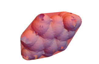
Geometric Features
Geometry affects how well molecules fit together and bond together. The atom positions of a molecule can be coupled with their van der Waals radii to construct a geometric mesh. For instance:
 rC = 170; rO = 152; rN = 155; rH = 120;
 chem = Entity["Chemical", "2Hydroxy4MethoxybenzoicAcid"];

 atomPos1 = chem["AtomPositions"];
 radii1 = chem["VertexTypes"] /. {"C" -> rC, "H" -> rH, "N" -> rN,
     "O" -> rO};
 rgn = RegionUnion[
    Table[Ball[atomPos1[[i]], radii1[[i]]], {i, 1, Length[atomPos1]}]];
 mesh = DiscretizeRegion[rgn];
 meshConvex = ConvexHullMesh[MeshCoordinates[mesh]];


 vMol = Volume[rgn];
 saMol = Area[RegionBoundary[mesh]];

 PPList = (List @@ BoundingRegion[mesh, "MinOrientedCuboid"])[[2]];
 vBox = Dot[Cross[PPList[[1]], PPList[[2]]], PPList[[3]]];
 saBox = 2*Total[Norm /@ (Cross @@@ Subsets[PPList, {2}])];
 edgesBox =
   Norm /@ ((List @@ BoundingRegion[mesh, "MinOrientedCuboid"])[[2]]);

 vConvex = Volume[meshConvex];
 saConvex = Area[RegionBoundary[meshConvex]];
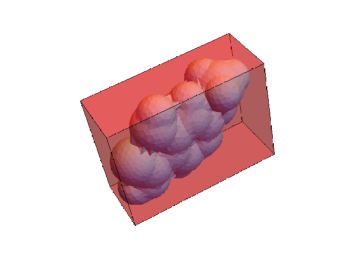
This extracts the volume and surface area of the mesh, minimum bounding box, and convex hull. These three meshes can be visualized.
mesh
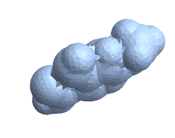
Show[RegionPlot3D[mesh, PlotStyle -> {LightBlue}, Boxed -> False],
 Graphics3D[{Opacity[0.4], Red,
   BoundingRegion[mesh, "MinOrientedCuboid"]}]]
Show[RegionPlot3D[mesh, PlotStyle -> {LightBlue}, Boxed -> False],
 RegionPlot3D[meshConvex, PlotStyle -> {Red, Opacity[0.4]}]]
Other Features
A number of other features are also extracted. Many of these are directly in ChemicalData[], such as molar mass, hydrogen bonding sites, rotatable bonds, bond tallies, etc. A more detailed list can be found in the preprocessing file on github.
Prediction
Melting Point
Primarily, I used these features to predict Melting Point, with mixed success. I used the predict function with random forest. The comparison plot is below:
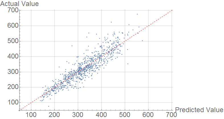
The mean average error is 30 K, outperforms the model of Karthikeyan & Glen. It is much higher than the error found by Lazzus, who used a small number of features both structural and quantum mechanical.
Boiling Point
Boiling point should be easier than melting point because the geometry of a molecule is less important. However, the random forest model performed fairly poorly, as shown in the comparison plot. 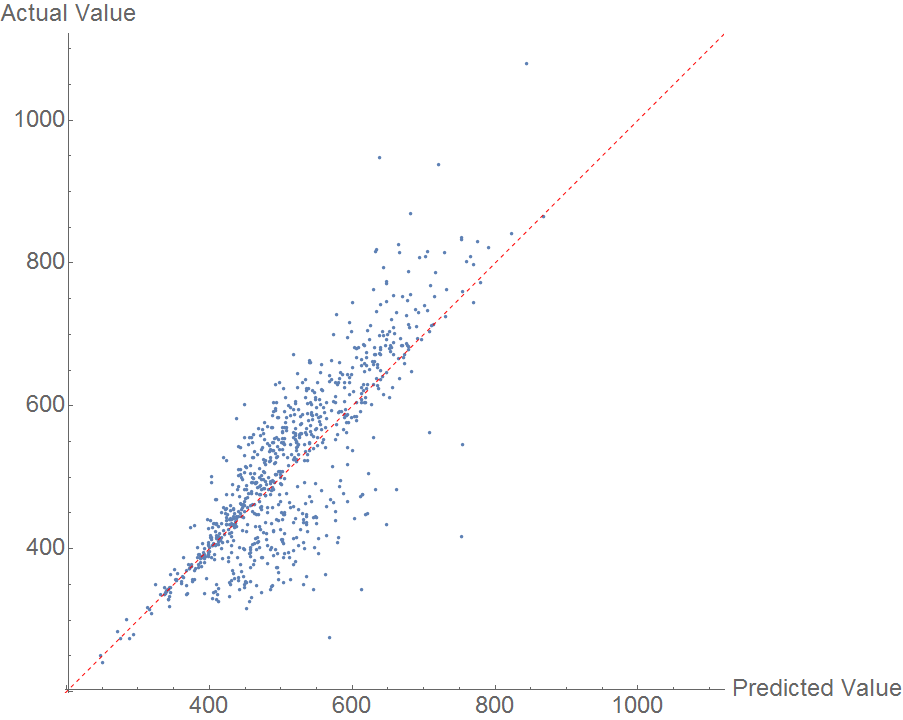
The data are not distributed randomly about the y=x line, indicating that there is likely another feature influencing the results. I'm interested to hear what features users suspect might be affecting boiling point. The MAE here is an outrageous 50 K.
Heat of Fusion
Using a similar prediction algorithm as above, the following comparison plot is produced. Because few compounds have heat of fusions measured, the sample size is smaller. Much like melting point predictions, there is a clear correlation, but the model does not fully explain the observations. 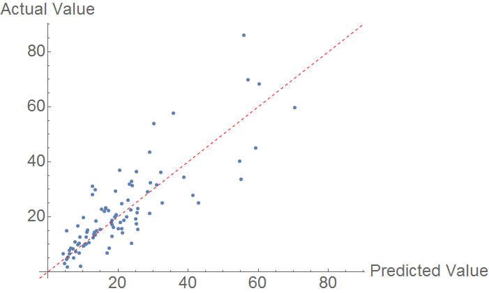
The MAE is mediocre, at around 6.18 KJ/Mol.
Heat of Vaporization
As enthalpy of vaporization is closely related to boiling point (See Trouton's Rule), it would be expected that the issues with boiling point would reappear in predicting heat of vaporization. However, this is not the case .
Prediction is done using a random forest model. The comparison plot is below. The data is immediately marked by a very prominent outlier, N-methyl pyrrole, with an actual heat of vaporization of 407 KJ/mol. This seems to be incorrect data, as NIST lists the heat of vaporization as 40.7 KJ/mol (see sources.) Aside from this outlier, the data is fairly well correlated, but as in the previous cases, the model is insufficient to fully predict heat of vaporization. 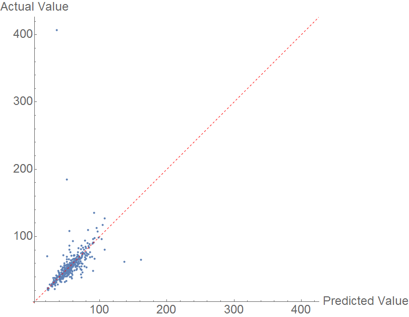
The MAE is once again mediocre, at 7.224 KJ/mol.
Heat of Combustion
Finally, heat of combustion is predicted using a similar model. The comparison plot resulting from the random forest algorithm shows fairly strong prediction, with a few significant outliers. Generally however, data points are very close to the perfect prediction line. 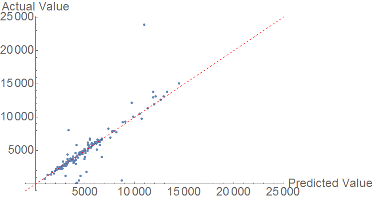
The MAE is 557.01 KJ/mol, but the data is generally much larger in magnitude.
Conclusion
Generally, it seems reasonable to approximate chemical properties from the structure alone. It would be interesting to see whether a well designed neural network is able to preform better than the random forest algorithm. To further improve the model, different features should be examined to explain the failure of prediction of boiling point. Additionally, I am curious if the model can be broadened to apply to organic molecules with other constituent elements, such as sulfur, phosphorous, and the halogens.
References
Winter, Mark. "The Periodic Table of the Elements." The Periodic Table of the Elements by WebElements. N.p., n.d. Web. 04 July 2017. https://www.webelements.com/.
Karthikeyan, M., Robert C. Glen, and Andreas Bender. "General Melting Point Prediction Based on a Diverse Compound Data Set and Artificial Neural Networks." Journal of Chemical Information and Modeling, vol. 45, no. 3, 2005, pp. 581-590.
"Theory: QSAR+ Descriptors." Accelrys, n.d. Web. 04 July 2017. http://www.ifm.liu.se/compchem/msi/doc/life/cerius46/qsar/theory_descriptors.html.
Katritzky, Alan, Mati Karelson, and Ruslan Petrukhin. "CODESSA PRO Classes of Descriptors." CODESSA PRO. N.p., n.d. Web. http://www.codessa-pro.com/descriptors/index.htm.
Lazzús, Juan A."Neural Network Based on Quantum Chemistry for Predicting Melting Point of Organic Compounds." Chinese Journal of Chemical Physics, vol.22, no.1, 2009, pp.19 - 26.
Rogers, David, and Mathew Hahn. "Extended-Connectivity Fingerprints." Journal of Chemical Information and Modeling, vol. 50, no. 5, 2010, pp. 742.
Libretexts. "Trouton's Rule." Chemistry LibreTexts. Libretexts, 09 Apr. 2017. Web. 05 July 2017. <a href="https://chem.libretexts.org/Core/Physical_and_Theoretical_Chemistry/Thermodynamics/Introduction_to_Thermodynamics/Trouton's_rule">https://chem.libretexts.org/Core/Physical_and_Theoretical_Chemistry/Thermodynamics/Introduction_to_Thermodynamics/Trouton's_rule.
Other thank you's: Peter Barendse, Mark Boyer, and Bob Nachbar


