Goal
My project was a simple investigation of the micro-macro link. In other words, my aim was to predict emergent behavior, macro-features of sandpiles, from local rules, sand redistribution rules at critical heights. I studied all variations of the Bak-Tang-Wiesenfeld sandpile model which are sand conserving and where each grain from avalanches is uniquely distributed, this includes critical heights from one to eight. This project was focussed on studying simple programs for the model rather than physical implications of the model.
Process
The sandpile model consists of a two-dimensional array with cell values that range from zero to the critical height. When the value of a cell exceeds the critical height the contents of that cell are redistributed among that cell's Moore neighbors (eight adjacent neighbors) according to a rule matrix, this event is called an avalanche. A trial consists of adding a single grain of sand (adding one) to the center cell of the array and allowing all avalanches to occur until the system reaches a fixed point. I investigated all 255 possible rules that met the constraints described in the previous section. In my later analysis I excluded the one rule with a critical height of eight, and the eight rules with a critical height of one because they all led to trivial behavior. I also excluded the 28 rules with critical height two because of limited computing resources. The piles generated by these rules extended over the edge of the table, and thus were not amenable to shape analysis. This left me with 218 rules to investigate. The main portion of my study was of piles with 3000 grains of sand on a 301 x 301 table for each rule. I measured the dimensions of the piles using ComponentMeasurements[ ].
Results
My initial qualitative observation was that many of the sandpiles exhibit a transient chaotic phase before settling to a periodic limit cycle.
I was able to accurately predict the growth direction of unidirectional sandpiles by creating a growth-vector. This vector is constructed by representing each 1 in a rule matrix as a vector. The sum of these vectors provides the growth-vector. Corner values are weighted by a factor of the square root of two and edge values by a factor of one. These factors are attributable to the square geometry of the table grid. Only unidirectional sandpiles (piles that grow in only one direction) can be described this way because sandpiles that grow in multiple directions have symmetric rulesets which produce growth-vectors of {0,0}.
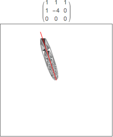
Example sandpile with corresponding rule matrix. Growth-vector is shown in red.
In addition to predicting the direction of growth I also made an effort to predict the rate of growth, thereby learning something of the overall shape of the sandpile (faster growth means longer elongated shape, slower means wider shape). Growth speed appeared to be related to the "spread" of 1s in the rule matrix, the magnitude of the growth-vector, and the critical height. The critical height is obviously a factor because it directly controls how frequently avalanches occur, and therefore how frequently growth occurs.
My first attempt at predicting "spread" was to calculate the total distance of 1s in the rule matrix from the growth-vector line. The thought was that a larger spread would correspond to a slower growth rate. I also weighted these calculations by multiplying by the absolute value of the critical heights. When ranked in descending order, this measure provided a sequence similar to the sequence obtained by ranking by increasing length. The length of each sandpile was measured with ComponentMeasurements[ ]. Certain pairs of piles however were interchanged in the ranking and piles with strictly diagonal rules (meaning all 1s in the rule matrices were only adjacent at corners) were improperly ranked. I attempted to account for this by dividing the speed metric by the magnitude of each growth-vector. This method was unsatisfactory.
My next attempt at predicting growth-rate was to use the same method as previously described, but to discount 1s in the rule matrix which lay behind the line that was orthogonal to the growth-vector and passed through the point {0,0}. The thought was that these grains were not contributing to the forward growth of the pile. The measure provided by this method was no more (if not less) satisfactory than the previous method which took into account all 1s in the rule matrix.
The next method was to calculate the intersection point of the growth-vector and an imagined bounding box (Line[{{1, 1}, {-1, 1}}], Line[{{-1, 1}, {-1, -1}}], Line[{{-1, -1}, {1, -1}}], Line[{{1, -1}, {1, 1}}]}). Then to calculate the total distance of all 1s in the rule matrix to this point. This value was then weighted in the same manners as described above. This method was also unsatisfactory.
The final and most successful method to predict growth rate and consequently an ordering of length was to calculate the average distance between all 1s in the rule matrix. The motivation for this method was reconsidering what would be an appropriate measure of "spread." All previous methods had obvious logical faults which partially stemmed by privileging some reference point or line from which the 1s in the rule matrix were spread from. The advantage of this method was that it provided a measure of how spread the 1s in the rule matrix were from themselves. The predicted ordering of length provided by this measure is very similar to that provided by measuring the sandpiles. Some neighbors in the ordering are interchanged and the strictly diagonal rules are still misplaced.
Conclusions
I found it is easy to predict the direction of sandpile growth in simple variations of the sandpile model. I also found it is possible to learn something about growth rate and resulting pile length, but the predictions are less precise. The improper ordering of neighbors is attributable to errors created by approximating the sandpiles as ellipsoids in the ComponentMeasurements[ ] function. These errors could possibly be avoided by measuring the length from the underlying table numerically. Still there remains the issue of precisely defining length. Possible definitions include the minimum and maximum extent of the column aligned with the growth-vector, or any vector parallel to the growth vector.
These simple programs were chosen for my investigation because they are entirely deterministic. A more difficult study would involve randomly choosing cells to add sand to, rather than always choosing the center cell. I provide functionality for this in my code and experimented with it some but did not investigate systematically. We know from autoplectic processes that simply because the models used were entirely deterministic with perfectly controllable initial conditions, does not mean they would be amenable to prediction. Another reason these programs were chosen is because only a single rule is ever applied. Consequently, I did not have to take into account complicated interactions between rules. Ultimately, studying the behavior of programs for simple models like the sandpile, help us develop a better understanding of the dynamics of micro-macro links.
Code
Setting Up Experiment
Set table size
tableSize = 100;

numberOfTrials = 500;

criticalHeight = 0;
Step
step[s_, rule_] := (
  (*n=n+Count[Flatten[UnitStep[s-criticalHeight]],
  1];*) (*comment in to count avalanches*)

  AppendTo[animation, table];
  Return[s +
    ListConvolve[rule, UnitStep[s - criticalHeight], 2,
     0]]) (*can also use ListCorrelate[]*)
Grain Adding Functions
addgrainCenter :=
  ReplacePart[
   table, {tableSize/2 + 1, tableSize/2 + 1} ->
    table[[tableSize/2 + 1]][[tableSize/2 + 1]] + 1];

addgrainRandom :=
  With[{x = RandomInteger[{1, tableSize + 1}],
    y = RandomInteger[{1, tableSize + 1}]},
   ReplacePart[table, {x, y} -> table[[x]][[y]] + 3]];
Pile Direction - Predicting pile direction from the rule set.
angleFunction = {-#[[1]] Sqrt[2] Sin[45 Degree] + #[[2]]*0 + #[[
       3]] Sqrt[2] Sin[45 Degree] - #[[4]]*1 + #[[5]]*1 - #[[6]] Sqrt[
       2] Sin[45 Degree] - #[[7]]*0 + #[[8]] Sqrt[2] Sin[
       45 Degree], #[[1]] Sqrt[2] Cos[45 Degree] + #[[2]]*1 + #[[
       3]] Sqrt[2] Cos[45 Degree] - #[[4]]*0 + #[[5]]*0 - #[[6]] Sqrt[
       2] Cos[45 Degree] - #[[7]]*1 - #[[8]] Sqrt[2] Cos[45 Degree]} &;

vector = angleFunction[DeleteCases[Flatten[#], -criticalHeight]] &;

angle = VectorAngle[
    angleFunction[DeleteCases[Flatten[#], -criticalHeight]], {0, 1}] &;

lines = Graphics@
    Line[{angleFunction[DeleteCases[Flatten[#], -criticalHeight]], {0,
        1}}] &;
Trial Function
trial[rule_] := (
  table = SparseArray[{}, {tableSize + 1, tableSize + 1}];
  (*aval = {};*) (*comment in to count avalanches*)
  (*n=
  0;*) (*comment in to count avalanches*)
  animation = {};
  Do[
   table = addgrainCenter;
   table = FixedPoint[step[#, rule] &, table];
   (*AppendTo[aval,n];*)(*comment in to count avalanches*)
   (*n=
   0;*) (*comment in to count avalanches*)
   , numberOfTrials];
  AppendTo[animation, table];
  ArrayPlot[Last@animation, PlotRange -> {0, criticalHeight},
   PlotLabel -> rule,
   Epilog -> {Red,
     Line[{1/2,
        1/2} + {60*vector@rule + tableSize/2, {tableSize/2,
         tableSize/2}}]}, AspectRatio -> 1])
Plotting
plotArrays := ArrayPlot[#, PlotRange -> {0, 7}] &;

increaseSize := (# /.
     Graphics[x__] :> Graphics[x, ImageSize -> 500]) &;
Rules
makeRule = x \[Function] {x :> a};
rules8cr4 =
  Flatten /@
   Map[makeRule,
    Subsets[Range[8], {4}], {2}]; (*enumerating all rules*)

rules8cr4 =
  ReplaceAll[
    Replace[{{1, 2, 3}, {4, -4, 5}, {6, 7, 8}}, rules8cr4, {2}],
    x_ /; x > 0 -> 0] /. a -> 1;

ruleChoose[n_, m_] := (
  partialrules =
   Flatten /@
    Map[makeRule,
     Subsets[Range[n], {m}], {2}]; (*enumerating all rules*)

  Return[ReplaceAll[
     Replace[{{1, 2, 3}, {4, -m, 5}, {6, 7, 8}}, partialrules, {2}],
     x_ /; x > 0 -> 0] /. a -> 1]
  )
Run Experiment
Permutations of Rules with Critical Height 7
criticalHeight = 7;
(*trial/@ruleChoose[8,7]*)(*comment in to run trial*)
Permutations of Rules with Critical Height 6
criticalHeight = 6;
(*trial/@ruleChoose[8,6]*)(*comment in to run trial*)
Permutations of Rules with Critical Height 5
criticalHeight = 5;
(*trial/@ruleChoose[8,5]*)(*comment in to run trial*)
Permutations of Rules with Critical Height 4
criticalHeight = 4;
(*trial/@ruleChoose[8,4]*)(*comment in to run trial*)
Permutations of Rules with Critical Height 3
criticalHeight = 3;
(*trial/@ruleChoose[8,3]*)(*comment in to run trial*)
Permutations of Rules with Critical Height 2
criticalHeight = 2;
(*trial/@ruleChoose[8,2]*)(*comment in to run trial*)
Permutations of Rules with Critical Height 1
criticalHeight = 1;
(*trial/@ruleChoose[8,1]*)(*comment in to run trial*)
Shape Analysis
Data - Here I am just collecting the data.
tables = Join[(3 - Reverse[((InputForm[#])[[1, 1, 1]])]) & /@
    v300t3000h3, (4 - Reverse[((InputForm[#])[[1, 1, 1]])]) & /@
    v300t3000h4, (5 - Reverse[((InputForm[#])[[1, 1, 1]])]) & /@
    v300t3000h5, (6 - Reverse[((InputForm[#])[[1, 1, 1]])]) & /@
    v300t3000h6, (7 - Reverse[((InputForm[#])[[1, 1, 1]])]) & /@
    v300t3000h7];

matrices =
  Join[MatrixForm[
      InputForm[#][[1, Position[InputForm[#][[1]], PlotLabel][[1, 1]],
        2]]] & /@ v300t3000h3,
   MatrixForm[
      InputForm[#][[1, Position[InputForm[#][[1]], PlotLabel][[1, 1]],
        2]]] & /@ v300t3000h4,
   MatrixForm[
      InputForm[#][[1, Position[InputForm[#][[1]], PlotLabel][[1, 1]],
        2]]] & /@ v300t3000h5,
   MatrixForm[
      InputForm[#][[1, Position[InputForm[#][[1]], PlotLabel][[1, 1]],
        2]]] & /@ v300t3000h6,
   MatrixForm[
      InputForm[#][[1, Position[InputForm[#][[1]], PlotLabel][[1, 1]],
        2]]] & /@ v300t3000h7];
Functions - These are functions to perform image analysis on the graphs in order to determine dimensions of the sandpile.
getMeasurements :=
  ComponentMeasurements[{Image[#], Clip[#]}, {"Centroid", "SemiAxes",
      "Orientation"}][[1, 2]] &;
getLengthWidth :=
  ComponentMeasurements[{Image[#], Clip[#]}, "SemiAxes"][[1, 2]] &;
g := Graphics[Rotate[Ellipsoid[#[[1]], #[[2]]], #[[3]]]] &;
Step 1 - Get measurement and generate ellipses to check accuracy of measurements later.
measures = getMeasurements /@ tables;
ellipses = g /@ measures;
Step 2 - Plot graphs and pair graphs with rule matrices and ellipses.
graphs = plotArrays /@ tables;
paired = MapThread[List, {tables, matrices, ellipses}];
Step 3 - Create matrix with measurements and data for analysis.
tableAndDim =
  MapThread[List, {graphs, matrices, getLengthWidth /@ tables}];

vectors =
  angleFunction[DeleteCases[Flatten[#[[2, 1]]], #[[2, 1, 2, 2]] ]] & /@
    tableAndDim;

tableAndDimAndVec =
  MapThread[
   List, {graphs, matrices, getLengthWidth /@ tables, vectors}];
Highlighting
highlightedPiles = HighlightImage[Image[#1], #3] & @@@ paired
Calculating Some Measure of Growth Rate
These are the points of the rule matrix.
points = {{-1, 1}, {0, 1}, {1, 1}, {-1, 0}, {0, 0}, {1,
    0}, {-1, -1}, {0, -1}, {1, -1}};
These functions generate the relevant points to a specific ruleset, and a line which intersects {0,0} and is in the direction of the sandpile growth vector.
relpointsFunc := DeleteCases[points*Flatten[#[[2, 1]]], {0, 0}] &
linesFunc := InfiniteLine[{#[[4]], {0, 0}}] &
Calculate distance from growth-vector line and box intersection point to each other point.
pointFromIntersect[x_] := (
  tvec = x[[4]];
  boxLines = {Line[{{1, 1}, {-1, 1}}], Line[{{-1, 1}, {-1, -1}}],
    Line[{{-1, -1}, {1, -1}}], Line[{{1, -1}, {1, 1}}]};
  intersection =
   Cases[Table[
     RegionIntersection[Line[{tvec, {0, 0}}], boxLines[[i]]], {i, 1,
      Length@boxLines}], Point[_]]
  )

intersectionDistances := Module[{points2, pointsFromIntersect},
  points2 = relpointsFunc /@ tableAndDimAndVec;
  pointsFromIntersect =
   pointFromIntersect[#][[1, 1, 1]] & /@ tableAndDimAndVec;

  Return[Table[
    Total[EuclideanDistance[pointsFromIntersect[[i]], #] & /@
      points2[[i]]], {i, 1, Length@points2}]]]
Calculates the average distance between all points.
avgDistances := Module[{pointsAD},
  pointsAD = relpointsFunc /@ tableAndDimAndVec;
  Return[Table[
    Total[EuclideanDistance @@@ Subsets[pointsAD[[i]], {2}]/
      Length@pointsAD[[i]]], {i, 1, Length@pointsAD}]]]
Calculates the average distance between all points, which are over line orthogonal to growth-vector line and intersecting with {0,0}
avgSelectDistances :=
 Module[{pointsASD, pointsOfInterestASD, finalPointsASD},
  pointsASD = relpointsFunc /@ tableAndDimAndVec;
  pointsOfInterestASD = pointFinder /@ tableAndDimAndVec;
  finalPointsASD =
   Table[Intersection[pointsASD[[i]], pointsOfInterestASD[[i]]], {i,
     1, Length@pointsASD}];

  Return[Table[
    Total[EuclideanDistance @@@ Subsets[finalPointsASD[[i]], {2}]/
      Length@pointsASD[[i]]], {i, 1, Length@finalPointsASD}]]]
Calculates the total distance from every point to growth-vector line.
getDistancesTotal := Module[{points, lines},
  points = relpointsFunc /@ tableAndDimAndVec;
  lines = linesFunc /@ tableAndDimAndVec;
  Return[Table[Total[RegionDistance[lines[[i]], #] & /@ points[[i]]]
    , {i, Length@lines}]]]
Calculates the total distance from every point, which is over line orthogonal to growth-vector line and intersecting with {0,0}, to growth-vector line.
pointFinder[x_] := (
  tvec = x[[4]];
  tortho = Which[
    tvec[[1]] == 0, {1, 0},
    tvec[[2]] == 0, {0, 1},
    tvec[[2]] =!= 0 && tvec[[1]] =!= 0, {tvec[[2]], -tvec[[1]]}];

  boxLines = {Line[{{1, 1}, {-1, 1}}], Line[{{-1, 1}, {-1, -1}}],
    Line[{{-1, -1}, {1, -1}}], Line[{{1, -1}, {1, 1}}]};
  dots = Cases[
    Union[Table[
      RegionIntersection[InfiniteLine[{tortho, {0, 0}}],
       boxLines[[i]]], {i, 1, Length@boxLines}]], Point[_]];

  slope = Which[
    tortho == {0, 1}, Infinity,
    tortho == {1, 0}, 0,
    tortho =!= {0, 1} && tortho =!= {1, 0}, tortho[[2]]/tortho[[1]]
    ];

  includedPoints = Select[points,
    Which[
     slope == Infinity && tvec[[1]] < 0, #[[1]] <= 0 &,
     slope == Infinity && tvec[[1]] > 0, #[[1]] >= 0 &,
     slope == 0 && tvec[[2]] < 0, #[[2]] <= 0 &,
     slope == 0 && tvec[[2]] > 0, #[[2]] >= 0 &,
     tvec[[1]] < 0 && tvec[[2]] > 0, #[[1]]*slope <= #[[2]] &,
     tvec[[1]] > 0 && tvec[[2]] < 0, #[[1]]*slope >= #[[2]] &,
     tvec[[1]] > 0 && tvec[[2]] > 0, #[[1]]*slope <= #[[2]] &,
     tvec[[1]] < 0 && tvec[[2]] < 0, #[[1]]*slope >= #[[2]] &
     ]
    ]
  )
(*Show[Graphics/@boxLines,Graphics[dots],Graphics[Point/@\
includedPoints]]*)

getDistances := Module[{lines, pointsD, pointsOfInterest, finalPoints},
  pointsD = relpointsFunc /@ tableAndDimAndVec;
  pointsOfInterest = pointFinder /@ tableAndDimAndVec;
  finalPoints =
   Table[Intersection[pointsD[[i]], pointsOfInterest[[i]]], {i, 1,
     Length@pointsD}];
  lines = linesFunc /@ tableAndDimAndVec;

  Return[Table[
    Total[RegionDistance[lines[[i]], #] & /@ finalPoints[[i]]]
    , {i, Length@lines}]]
  ]
All Positive Projections
positiveProjections := Module[{pointsAgain},
  pointsAgain = relpointsFunc /@ tableAndDimAndVec;
  dotProducts =
   Table[Total[
     Select[(Dot[#, vectors[[i]]]/Norm[vectors[[i]]] &) /@
       pointsAgain[[i]], Positive]], {i, 1, Length@vectors}]
  ]
Analysis
Rate (referred to as speed here) by chosen measure.
speed = avgDistances;

(* Options for Measurement *)

(*
avgDistances;
intersectionDistances;
getDistances;
getDistancesTotal;
avgSelectDistances;
positiveProjections;
*)
Speed weighted by critical height and/or magnitude of growth-vector.
weightedSpeed =
  Table[N@Abs[(speed[[i]]) matrices[[i, 1, 2, 2]]](*/Norm[vectors[[
   i]]]*), {i, 1, Length@speed}];
Combining Data
tableAndDimAndVecAndDist =
  MapThread[
   List, {graphs, matrices, getLengthWidth /@ tables, vectors,
    N[speed, 2], N[weightedSpeed, 2]}];

SortBy[tableAndDimAndVecAndDist, #[[3, 1]] &] //
  Column; (*sort by height is [[3,1]], sort by width is [[3,2]]*)
Organizing and Sorting Data
Multicolumn[{SortBy[
   Select[tableAndDimAndVecAndDist, #[[4]] =!= {0, 0} &], #[[3,
     1]] &], Reverse[
   SortBy[Select[
     tableAndDimAndVecAndDist, #[[4]] =!= {0, 0} &], #[[5]] &]]}, 2]
Some Plots
(*Line Plot of Heights*)
ListPlot[Sort[(getLengthWidth /@ tables)[[All, 1]]],
 AxesLabel -> "Length"]

(*Line Plot of Widths*)
ListPlot[Sort[(getLengthWidth /@ tables)[[All, 2]]],
 AxesLabel -> "Width"]
Animation
tableSize = 60;
numberOfTrials = 2000;
criticalHeight = 4;
trial@{{1, 1, 0}, {1, -4, 0}, {0, 1, 0}};

ListAnimate[ArrayPlot[#, PlotRange -> {0, 4}] & /@ animation, 900]
GitHub
Repo
 Attachments:


