Exon Prediction

(link to project)

Context

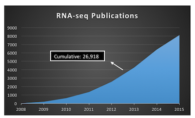
Advances is sequencing technology has resulted in a boom of genomic data (fig 1). Despite the terabytes (TBs) of sequence data, biologists are far from understanding the complexity of the human genome. For example, RNA-seq studies allow bioinformatics to discern differentially expressed genes (DEGs) and differentially expressed exons (DEEs) between two or more groups (e.g. control, treatment).

Fig 1: The rise of RNA-seq publications

To review, genes consist of exons and introns, were the former are the coding regions (may become part of the final protein) and the latter are riffled between exons and not included in the protein (fig 2.)

Fig 2: Exonic structure of a gene

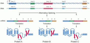
Despite having access to both DEGs and DEEs these RNA-seq studies almost exclusively focus on DEGs with less than 2% mentioning DEEs. This might stem from the fact that the exome (collection of exons within the human genome) is not as well annotated as the genes of the genome. Nonetheless, differential use of exons in alternate splicing - the use of different exons of a given gene to produce different proteins (see fig 2) - is disease relevant (e.g. gene ACTN4 preferentially expressed exon 8a in the kidney - mutations in which results in familial focal segmental glomerulosclerosis).

Thus given the disease relevance it would be beneficial to improve the annotation and understanding of the exome. Here such is attempted via deep learning.

Prerequisites

I will be taking advantage of the suite bedtools for sequence extraction. This must be installed. In addition, it will be required in your path later on, so run SetEnvironment["PATH" -> Import["!source ~/.bash_profile; echo $PATH", "Text"]]

Data acquisition

One can obtain the file hg38.fa (annotated human genome) from UCSC's Genome Browser. There one can also obtain a list of know exonic and intronic regions. Given the size of these files, they are not included in this post.

Data Preprocessing

A large portion of this post is dedicated to the pre-processing of the genomic data. As we will be using a convolutional neural network (which requires fixed input length) we must be able to:

1. get the desired DNA sequences from the genome (e.g. exons)
2. ensure that our sequences are within a fixed length
3. randomly select sequences from our dataset
4. 'pad' our sequences to a set length (length of our input) with the actual adjacent nucleotides

while not exactly hard handling the large file size requires line-by-line processing. Thus I will walk through the pre-processing pipeline

FileLines

As some of these files are quite large such that one may not be able to import the entire thing into their notebook, I will be using OpenRead[] and OpenWrite[]. Thus it would be handy to know how many lines are in our files. While one could use Run[wc -l <file>], the following does the equivalent (albeit somewhat slower) in Mathematica:

ClearAll[FileLines]
FileLines::usage = 
  "FileLines returns the number of lines in the given file.";
FileLines::dne = "File '`1`' does not exist.";
FileLines[file_String] /; ! FileExistsQ[file] := (Message[
   FileLines::dne, file]; $Failed)
FileLines[file_String] := 
 Length@ReadList[file, Null@String, NullRecords -> True]

convertBed

The list of exonic and intronic regions will be supplied in .bed file format, a tab delimited file with three mandatory fields and several optional ones (read more about the BED format here). I will be using the first six fields:

1. Chromosome (on which chromosome the sequences appears)
2. Start (index of where the sequence starts)
3. Stop (index of where the sequence stops)
4. Name (name of the sequence)
5. Score (a score used by the genome browser for coloration)
6. Strand (on which strand of DNA +/- the sequence is on)

The code for converting your bed files into a dataset follows:

(* give a readble name to what could be an anonymous function for \
ensuring strings are output correctly *)

wrapInQuotes[item_] := "\"" <> item <> "\"";
(* Convert a BED file to a Mathematica association *)

convertBED::usage = 
  "Converts the given file to a an association and outputs it to a \
file with the same name with the extension '.m'.";
convertBED[bedFile_] := Module[
  {fileLines = FileLines[bedFile],
   outputStream, line, lineIndex, inputStream, bed},

  (* Close files in case they are somehow already open *)

  Quiet[Close[bedFile]];
  Quiet[Close[FileBaseName[bedFile] <> ".m"]];

  (* If fileLine fails, file does not exist. Fail this evaluation*)

  If[fileLines == $Failed, $Failed];

  (* Open the output stream *)

  outputStream = OpenWrite[FileBaseName[bedFile] <> ".m"];

  (* Start a list *)
  WriteString[outputStream, "Dataset[{"];
  (* Open the input stream *)
  inputStream = OpenRead[bedFile];

  (* Give the user a way to monitor the progress *)
  Monitor[
   lineIndex = 1;
   While[lineIndex <= fileLines,
    line = ReadLine[inputStream];
    If[line === EndOfFile, Break[]];
    line = StringSplit[line, "\t"];

    bed = <|wrapInQuotes@"Chromosome" -> wrapInQuotes@line[[1]], 
      wrapInQuotes@"Start" -> line[[2]], 
      wrapInQuotes@"Stop" -> line[[3]], 
      wrapInQuotes@"Name" -> wrapInQuotes@line[[4]], 
      wrapInQuotes@"Score" -> wrapInQuotes@line[[5]], 
      wrapInQuotes@"Strand" -> wrapInQuotes@line[[6]]|>;

    (*WriteString[outputStream,ToString[wrapInQuotes/@line]];*)

    WriteString[outputStream, ToString@bed];
    If[lineIndex < fileLines, WriteString[outputStream, ","];];

    lineIndex += 1;
    ]

   , ProgressIndicator[lineIndex, {1, fileLines}]
   ];

  (* End the list *)
  WriteString[outputStream, "}]"];
  (* Close Streams *)
  Close[inputStream];
  Close[outputStream];
  ]

Note: one could replace wrapInQuotes with ToString[<symbol>,InputForm].

BED Dataset helpers

For extracting sequences we would like to be able to: 1. get sequences at random, and 2. select sequences within a length falling within a given closed interval

While neither of these functions actually warrant their existence, for readability they are included below:

(* A readable wrapper for an otherwise not needed function *)
randomSampleSequences[dataset_Dataset, number_Integer] := 
 RandomSample[dataset, number]

(* A readable wrapper for an otherwise not needed function *)
filterSequencesWithLength[data_, minLength_, maxLength_] := 
 data[Select[minLength <= #Stop - #Start <= maxLength &]]

Padding sequences

With our bed files converted to Datasets and some helper functions for filtering sequences of a given length as well and randomly sampling those sequences, we next would like the ability to pad all of our sequences to a given length. This will require us knowing how long the sequence's chromosome's length (as a sequence padded beyond that length will be meaningless). Acquiring this information is trivial (using the hg38.fa file, simply get the length of each chromosome). In addition the following function assumes that chromosome lengths are stored as a dataset, e.g. (Dataset[{<|chr1->n|>,...}].

padSequences::usage = 
  "padSequences[sequenceData, chromosomeLengths, padTo]:\n\t\
sequenceData:\t\ta Dataset of sequences\n\tchromosomeLengths:\ta \
Dataset of chromosome lengths\n\tpadTo:\t\t\tan integer of how long \
each sequence in sequenceData should be.\n\npads all the sequences in \
sequenceData into a set length.";
padSequences[sequenceData_Dataset, chromosomeLengths_Dataset, 
  padTo_Integer] := Module[
  {upstream, downstream, nucleotidesNeeded, length},
  sequenceData[
   All,
   <|
     "Chromosome" -> #["Chromosome"],
     length = #["Stop"] - #["Start"];

     (* How many NTs are needed to make exon specified length *)

     nucleotidesNeeded = padTo - length;

     (* Randomly select an integer in that range to pad upstream *)

        upstream = RandomInteger[{1, nucleotidesNeeded}];


     (* If start - upstream < 1, update upstream to start at 1 *)

      If[ #["Start"] - upstream < 1, upstream = #["Start"] - 1];

     (* Set downstream as the remainder of needed - upstream *)

     downstream = (nucleotidesNeeded - upstream);

     (* If stop + downstream > chromosomeLength, shift *)

     If[#["Stop"] + downstream > chromosomeLengths[#[[1]]], 
      downstream = chromosomeLengths[#["Chromosome"]] - #["Stop"]; 
      upstream = (nucleotidesNeeded - downstream)];


     "Start" -> #["Start"] - upstream,
     "Stop" -> #["Stop"] + downstream,
     "Name" -> "Padded_" <> #["Name"],
     "Score" -> #["Score"],
     "Strand" -> #["Strand"]
     |> &
   ]
  ]

Extracting sequences from the genome

Finally with our filtered, randomly sampled, padded sequences (in bed format) we are finally ready to extract the raw nucleotides from the genome. This requires use of bedtools. To keep the project within Mathematica, each component (arguments, options, etc) of the bedtool function are stored as variables and stringed together.

extractSequences::usage = 
  "extractSequences[referenceFile, bedFile, outputFile]:\n\t\
referenceFile:\tfile of the reference genome\n\tbedFile:\t\ta file \
containg the start/stop locations of regions to extract from \
referenceFile\n\toutputFile:\t\ta file in which to store the \
extracted sequences.\n\nThis function requires bedtools.";
extractSequences[referenceFile_, bedFile_, outputFile_] :=
  Module[
   {fastaFromBed, fastaInput, bed, fastaOut, forcedStrandedness, 
    named, tabbed, command},
   fastaFromBed = "fastaFromBed ";
   fastaInput = "-fi ";
   bed = "-bed ";
   fastaOut = "-fo ";
   forcedStrandedness = "-s ";
   named = "-name ";
   tabbed = "-tab ";
   command = 
    fastaFromBed <> fastaInput <> referenceFile <> " " <> bed <> 
     bedFile <> " " <> fastaOut <> outputFile <> " " <> 
     forcedStrandedness <> named <> tabbed;
   Run[command]
   ];

This will result in a tab delimited FASTA file. While nice, it would be preferential to have our file as a dataset. The following achieves this:

FastaTabToDataset::usage = 
  "Converts the output of a 'fastaFromBed <args> -tab' command to a \
Mathematica Dataset.";
FastaTabToDataset[fastaFile_] := Module[
  {fileLines = FileLines[fastaFile],
   outputStream, line, lineIndex, inputStream, output, annotation},

  (* Close files if they were otherwise open *)

  Quiet[Close[fastaFile]];
  Quiet[Close[FileBaseName[fastaFile] <> ".m"]];

  (* If fileLine fails, file does not exist. Fail this evaluation*)

  If[fileLines == $Failed, $Failed];

  (* Open the output stream *)

  outputStream = OpenWrite[FileBaseName[fastaFile] <> ".m"];


  (* Start a list *)
  WriteString[outputStream, "Dataset[{"];
  (* Open the input stream *)
  inputStream = OpenRead[fastaFile];

  (*Display a handly ProgressIndicator*)
  Monitor[
   lineIndex = 1;
   While[lineIndex <= fileLines,
    line = ReadLine[inputStream];
    If[line === EndOfFile, Break[]];
    line = StringSplit[line, "\t"];


    annotation = "Sequence";
    If[StringContainsQ[line[[1]], "exon"], annotation = "Exon"];
    If[StringContainsQ[line[[1]], "intron"], annotation = "Intron"];


    output = <|wrapInQuotes@"Name" -> wrapInQuotes@line[[1]],
      wrapInQuotes@"Sequence" -> wrapInQuotes@ToUpperCase@line[[2]],
      wrapInQuotes@"Class" -> wrapInQuotes@annotation|>;

    (*WriteString[outputStream,ToString[wrapInQuotes/@line]];*)

    WriteString[outputStream, ToString@output];
    If[lineIndex < fileLines, WriteString[outputStream, ","];];

    lineIndex += 1;
    ]

   , ProgressIndicator[lineIndex, {1, fileLines}]
   ];


  (* End the list *)
  WriteString[outputStream, "}]"];
  (* Close Streams *)
  Close[inputStream];
  Close[outputStream];
  ]

With our raw sequences extracted from the genome we are now ready to focus on the neural network!

Wrapper for the preprocessing pipeline

As including all these steps might be obnoxious one can wrap it all into a nice function with progress indicators as follows:

generateTrainingSet[
  "Exon" -> <|"Data" -> edata_, "Min" -> emin_, "Max" -> emax_|>,
  "Intron" -> <|"Data" -> idata_, "Min" -> imin_, "Max" -> imax_|>,
  "Samples" -> samples_, "PaddingLength" -> paddingLength_, 
  "ChromosomeLengths" -> chromosomeLengths_] := Module[
  {
   filteredExons, filteredIntrons,
   randomExons, randomIntrons,
   paddedExons, paddedIntrons,
   trainingExons, trainingIntrons,
   trainingData, dummyTimeStep = 0, temp
   },
  Monitor[

   (*Filter Exons*)
   dummyTimeStep += 1;
   temp = PrintTemporary["Filtering Exons"];
   filteredExons = filterSequencesWithLength[edata, emin, emax];
   NotebookDelete[temp];

   (*Filter Introns*)
   dummyTimeStep += 1;
   temp = PrintTemporary["Filtering Introns"];
   filteredIntrons = filterSequencesWithLength[idata, imin, imax];
   NotebookDelete[temp];

   (*Sample Exons*)
   dummyTimeStep += 1;
   temp = PrintTemporary["Sampling Exons"];
   randomExons = randomSampleSequences[filteredExons, samples];
   NotebookDelete[temp];

   (*Sample Introns*)
   dummyTimeStep += 1;
   temp = PrintTemporary["Sampling Introns"];
   randomIntrons = randomSampleSequences[filteredIntrons, samples];
   NotebookDelete[temp];

   (*Padding Exons*)
   dummyTimeStep += 1;
   temp = PrintTemporary["Padding Exons"];
   paddedExons = 
    padSequences[randomExons, chromosomeLengths, paddingLength];
   NotebookDelete[temp];

   (*Padding Introns*)
   dummyTimeStep += 1;
   temp = PrintTemporary["Padding Introns"];
   paddedIntrons = 
    padSequences[randomIntrons, chromosomeLengths, paddingLength];
   NotebookDelete[temp];

   (*Export Padded BED File*)
   dummyTimeStep += 1;
   temp = PrintTemporary["Exporting padded sequences"];
   Export["padded_training_data.txt",
    Join[
     Normal@Normal@paddedExons[Values],
     Normal@Normal@paddedIntrons[Values]
     ], "TSV"];
   NotebookDelete[temp];

   (*Extract Sequences from Genome*)
   dummyTimeStep += 1;
   temp = PrintTemporary["Extracting padded sequences from genome"];
   extractSequences["hg38.fa", "padded_training_data.txt", 
    "training_data.fa"];
   NotebookDelete[temp];

   (*Convert Sequences to Dataset*)
   dummyTimeStep += 1;
   temp = PrintTemporary["Converting sequences to Dataset"];
   FastaTabToDataset["training_data.fa"];
   NotebookDelete[temp];

   (*Load Sequence Dataset*)
   dummyTimeStep += 1;
   temp = PrintTemporary["Loading Sequence Dataset"];
   trainingData = Get@"training_data.m";
   NotebookDelete[temp];

   , ProgressIndicator[dummyTimeStep, {1, 10}]
   ];

  Return[trainingData];
  ]

e.g. one might call:

trainingData = generateTrainingSet[
   "Exon" -> <|"Data" -> exons, "Min" -> 200, "Max" -> 500|>,
   "Intron" -> <|"Data" -> introns, "Min" -> 600, "Max" -> Infinity|>,
   "Samples" -> 180000, (* number of samples to retrieve of each (e.g. trainingData will be size 2n *)
   "PaddingLength" -> 600, 
   "ChromosomeLengths" -> chromosomeLengths
   ];

In addition, some sequences have the nucleotide "N" (e.g. unsequenced). It is best to filter these out:

filteredTrainingSet = 
  trainingData[
   Select[With[{chars = Characters@#Sequence}, 
      AllTrue[(StringContainsQ[#, ("A" | "T" | "G" | "C")] & /@ 
         chars), # == True &]] &]];

With our training data complete, one should break the data into training, validation and test sets. Following, one can rename the dataset to be compatible with NetTrain as follows:

trainingSet = 
  trainingSet[
   All, <|"Input" -> #["Sequence"], "Output" -> #["Class"]|> &];
validationSet = 
  validationSet[
   All, <|"Input" -> #["Sequence"], "Output" -> #["Class"]|> &];
testSet = 
  testSet[All, <|"Input" -> #["Sequence"], 
     "Output" -> #["Class"]|> &];

Neural Network

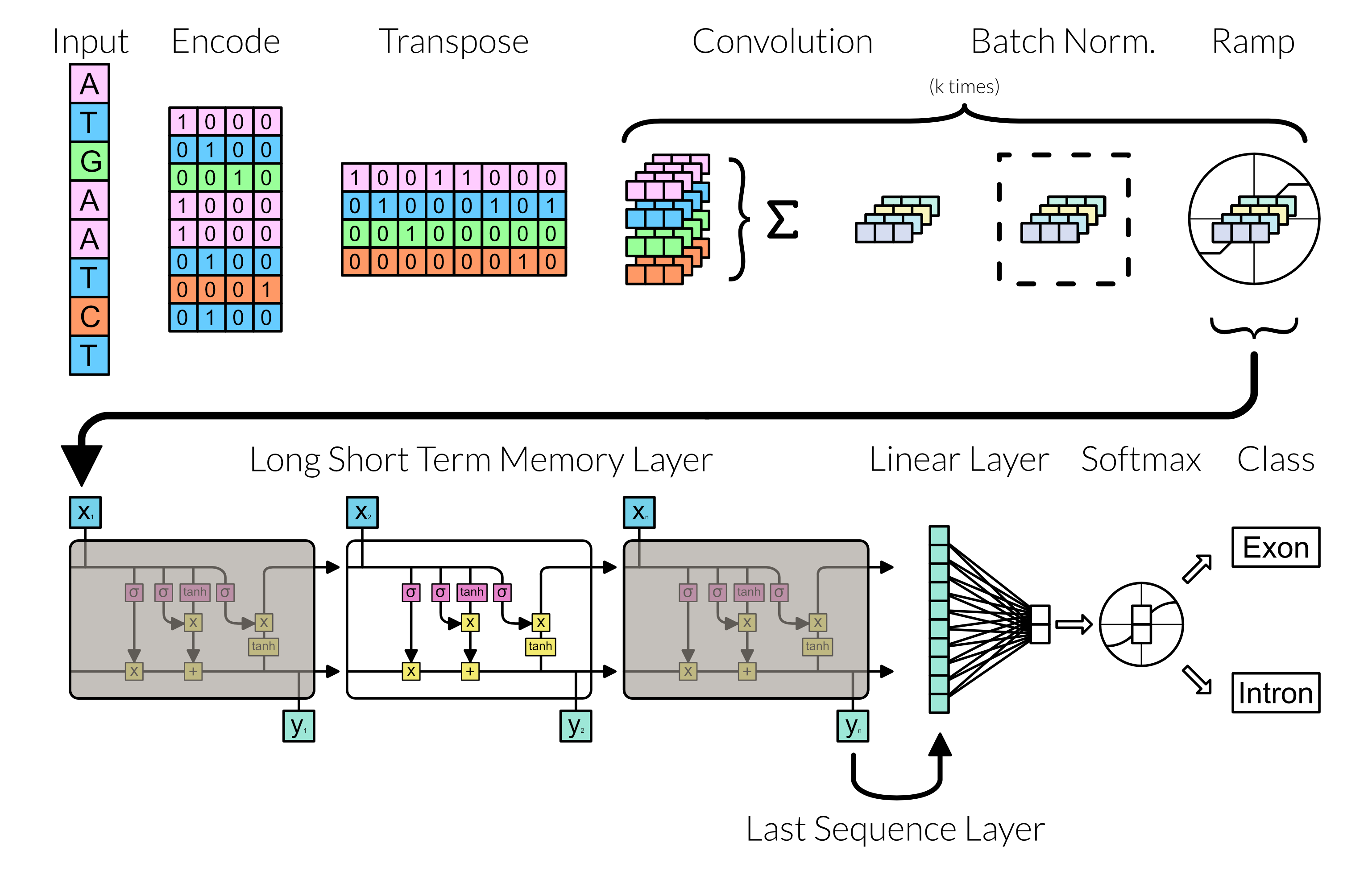
With the grunt of preprocessing finish, we can focus on making the neural network. Here the neural network follows the following diagram:

Fig 3: Network Architecture

Convolution

To handle the convolution chuck of the network the following code encapsulates the repetitive aspects of the structure.

Convolution Block

Clear[convolutionBlock]
convolutionBlock::usage="Basic convoultion neural network architecture modified for handing sequences of strings. Returns a NetChain as follows:\n\tConvolutionLayer --> BatchNormalizationLayer --> ReshapeLayer --> ElementwiseLayer";
convolutionBlock[
"Channels"->channels_,
"Kernel"->kernel_,
"SequenceLength"->seqLen_,
convOpts___
]:=NetChain[{
ConvolutionLayer[channels,kernel,convOpts],
ReshapeLayer[{channels,seqLen,1}],
BatchNormalizationLayer[],
ReshapeLayer[{channels,seqLen}],
ElementwiseLayer[Ramp]
}]

Residual Convolution Block Chain

 residualConvolutionalChain[
"Channels"->channels_,
"Kernel"->kernel_,
"SequenceLength"->seqLen_,
"PaddingSize"->pad_,
"InitalStride"->initStride_,
"ChainLength"->chainLen_,
convOpts___]:=Module[
{nonDownsizedConvolutionBlocks=chainLen-1,netGraph,netGraphConnections,downsizedConvolutionBlock},
(* Create the downsized cnn block *)
downsizedConvolutionBlock=convolutionBlock["Channels"->channels,"Kernel"->kernel,"SequenceLength"->seqLen,"PaddingSize"->pad,"Stride"->initStride,convOpts];

(* Start a NetGraph with the downsized cnn block *)
netGraph={downsizedConvolutionBlock};

(* Table non-downsized blocks for {i,chainLen-1} and append to the netGraph *)
Table[
AppendTo[
netGraph,
convolutionBlock["Channels"->channels,"Kernel"->kernel,"SequenceLength"->seqLen,"PaddingSize"->pad,"Stride"->1,convOpts]
],{i,nonDownsizedConvolutionBlocks}
];

(* Add the TreadingLayer to enable the residual architecture *)
AppendTo[netGraph,ThreadingLayer[Plus]];

(* Specify the residual architecture *)
netGraphConnections=Flatten[Join[Table[i->i+1,{i,chainLen}],{1->chainLen+1}]];
(* Return NetGraph*)
NetGraph[netGraph,netGraphConnections]
]

Defining the Network

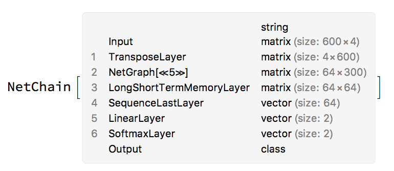
With the helper functions defined our network can be made as follows:

net=NetInitialize[
    NetChain[{
       TransposeLayer["Input"->{600,4}],
       residualConvolutionalChain[
         "Channels"->64,"Kernel"->{3},"SequenceLength"->300,
         "PaddingSize"->1,"InitalStride"->2,"ChainLength"->4
       ],
       LongShortTermMemoryLayer[64],
       SequenceLastLayer[],
       (*AggregationLayer[Mean],*)
       LinearLayer[2],
       SoftmaxLayer[]
    },
       "Input" -> NetEncoder[{"Characters", "ATCG", "UnitVector"}],
       "Output" -> NetDecoder[{"Class", {"Exon", "Intron"}}]
    ]
];

which can then be trained utilizing a GPU

trainedNet=
NetTrain[
    net,
    trainingSet,
    ValidationSet->validationSet,
    TargetDevice->"GPU",
    (*MaxTrainingRounds\[Rule]200,*)
    Method->{"ADAM","LearningRate"->0.0001},
    (* Output Learning Rate (not needed if set via Method Option )*)
    TrainingProgressFunction->{
       Function[
         If[
          #Batch===1&&#Round===1,
          Print["\n\nInitial Learning Rate:\t"<>ToString[MXNetLink`$LastInitialLearningRate]<>"\n\n"],
          Null
         ]
       ]
       ,"Interval"->Quantity[1,"Batches"]
    }
];

Measurements

The measurements of accuracy can be obtained via ClassifierMeasurements cmTest=ClassifierMeasurements[trainedNet,cmDataset[testSet]]; cmTrain=ClassifierMeasurements[trainedNet,cmDataset[testSet]];

where cmDataset converts a Dataset into a list of rules for ClassifierMeasurements:

cmDataset[networkData_Dataset]:=(Rule@@Normal[#][[All,2]])&/@Normal[networkData]

Results

The training this network yielded a model that had ~87% accuracy on the test set and 89% accuracy on the training suggesting that the model does not over fit the training set.

Conclusions

Recently deep neural networks used in biology utilized CNNs on known sequence features. Here it is show that deep learning is robust enough to handle raw DNA sequences with adequate performance. While promising more work is required to find out just how sufficient this network is at exon prediction. Given that our classifier was binary (exon or intron), it may have learned only to distinguish between the two and not necessary learned how to identify an exonic sequence in DNA.

Future Directions

1. Utilize known genomic features to improve the model. Such features include ORF, codon bias, protein distribution, exon splicing enhancers / silencers (ESE / ESS) (ESEs can be readily found, e.g. http://genes.mit.edu/burgelab/rescue-ese/ESE.txt), etc.

2. Slide throughout the entire human genome to identify novel exons (not including those in our initial data set). With candidate exons found, utilize the TBs of RNA-seq reads to validate candidates as unannotated exons and subsequently annotate them.

3. Exons have a wide range in length, from micro exons at 2 NTs to the longest know exon at over 200,000 NTs. A variant of this model should be made for small and large exons.

4. Include known non-coding, non-exon, non-intron regions in the learning process and see if performance can be maintained if not augmented.