Background

George Cybenko showed in 1989 that in principle a feed-forward neural network with an hidden layer containing a finite number of neurons can approximate continuous functions on compact subsets of $\mathbb{R}^n$. This meant that neural networks could be employed to solve hithero difficult to solve differential equations. However the logistics of this were/are not very clear. Here I have attempted to understand how effective neural networks are in approximationg continuous real valued functions.

Approximating Bessel functions

One of the most well known of the special functions, these are the solutions of Bessel's equation and frequently appears in many different branches of physics. These are oscillatory functions with constantly varying amplitudes.

Plot[BesselJ[1, x], {x, -8, 8}]

![enter image description here

Now I will approximate it using a neural network. My network of choice is

sinNet = NetChain[{LinearLayer[30], Sin, LinearLayer[20], Sin, 
   LinearLayer[1]}, "Input" -> "Real", 
  "Output" ->  NetDecoder["Scalar"]]

This is a network with three hidden layers with a sinusoidal activation function associated to two of them. Before I can use it to approximate the Bessel function I will have to train it. For that purpose I generate some training and validation data.

dataBessel = (# -> BesselJ[1, #]) &@ RandomReal[{-8, 8}, 50000];
validationBessel = (# -> BesselJ[1, #]) &@ RandomReal[{-8, 8}, 200];

And now the training.

{trainedSinNet, validationLossListS, batchLossListS} = 
  NetTrain[sinNet, dataBessel, 
   Automatic, {"TrainedNet", "ValidationLossList", "BatchLossList"}, 
   ValidationSet -> {validationBessel, 
     "Interval" -> Quantity[1, "Rounds"]}, MaxTrainingRounds -> 100, 
   TrainingProgressReporting -> {plotSolution[#Net, #AbsoluteBatch] &,
      "Interval" -> 0.3}];

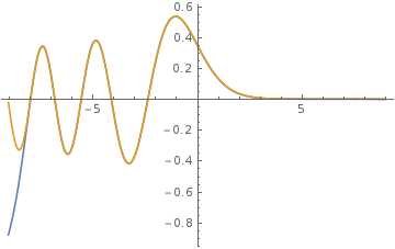
The TrainingProgressReporting option helps to visulize the training porcess. After training for a 100 rounds we get the following.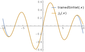

Not too shabby, huh! Sure it deviates quite a bit beyond the boundaries of the training data, but in that range the result is commendable. Now one can say that this is overfitting. But the training data set was random. So the neural network at least did a good job of interpolating the function in between the boundaries of the training dataset. The thing to note here is that this is a stochastic process and so results will vary somewhat each time. However as long as the errors are within tolerance in the region of interest it should be fine. In fact we can to estimate how bad it performs over a series of trials. I will consider to different metrics to enumerate the perfomance, one is the root mean square of the difference between the approximated and the actual values of the function and the other is the maximum difference between the approximated and the actual values of the function.

besselSinRMSE = {}; besselSinMax = {};

Table[{trainedSinNet = 
    NetTrain[sinNet, dataBessel, ValidationSet -> validationBessel, 
     MaxTrainingRounds -> 100]; 
   AppendTo[besselSinRMSE, 
    RootMeanSquare[trainedSinNet[#] - BesselJ[1, #] &@ $refRange]]; 
   AppendTo[besselSinMax, 
    Max[trainedSinNet[#] - BesselJ[1, #] &@ $refRange]];}, 30];
<< "ErrorBarPlots`"
ErrorListPlot[
 Table[{besselSinRMSE[[i]], StandardDeviation[besselSinRMSE]}, {i, 1, 
   Length[besselSinRMSE]}], ErrorBarFunction -> Automatic]

ErrorListPlot[
 Table[{besselSinMax[[i]], StandardDeviation[besselSinMax]}, {i, 1, 
   Length[besselSinMax]}], ErrorBarFunction -> Automatic]

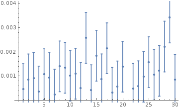
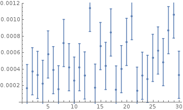
The root mean square error was generally between $10^{-4}$ and $10^{-3}$ and the maximum error was of the order of $10^{-3}$. We can also try to approximate other functions and we can even use activation functions other than the sinusoidal one. Here are the results of some of those that I tried.

Approximation of Scorer function

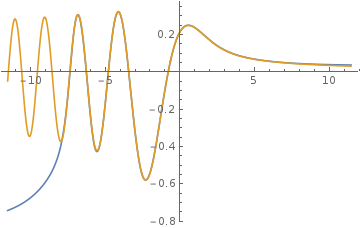
For this one I had used tanh instead of sin as the activation function. Again the result shows a significant similarity with the actual function within the boundaries of the training data set.

Approximation of Airy function

This is with a Gaussian activation function.

Source

You can find my notebook on github.

Future work

• I plan to work on improving the behaviour at the boundaries (not quite sure about how).
• Generalise this to continuous real-valued functions of multiple variables.
• Use this function approximation ability of neural networks to solve differential equations.