*"[...] we always found that the spaces traversed were to each other as the squares of the times, and this was true for all inclinations of the plane"* Galileo Galilei Dialogues Concerning Two New Sciences, 1638
Part 0. Introduction
The goal of this project is to the develop a STEM learning unit for secondary school students mixing mathematics, science and coding. With this work I want to reproduce (taking data from the real world) the Galileo inclined plane experiment, and analyze it with the Wolfram Language to deduce the physical law of falling bodies. This three week project at WSS17 will be part of a bigger educational project. Because I expect to start a series of open learning materials for sharing and contributing to the Computer-Based Math , the Wolfram Demonstration Project and the Computational Thinking Initiative.
In 1604 Galileo realized one of his most famous discoveries with the inclined plane experiment. In this experiment he measured the distance a ball rolls down a ramp for each unit of time. He presents his results in the 1638 book Dialogues concerning Two New Sciences, where it describes the law of motion of falling bodies without friction. At the image below you can read a fragment from the 1638 Galileo's book Dialog Concerning Two New Sciences (translated by Henry Crew and Alfonso de Salvio, Macmillan 1914).
And in Wikipedia we can find a good source of information about Galileo and the equations of motion on an inclined plane:
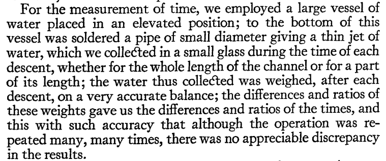
One of the most difficult questions of the Galileo experiment was how to measure the lapsed time for the falling body at different heights. We must think that the experiment was done in the 17th century and at the time there weren't cronometers to compute time. For that purpose Galileo used a kind of water clock device. Therefore, measuring the weight of the water with precision it can be deduced the value of the time because it is directly proportional to the weight of the dropped water.
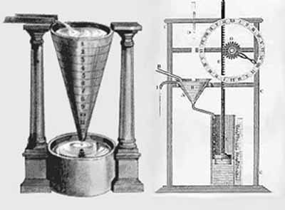
In the following video the historical experiment is explained with details:
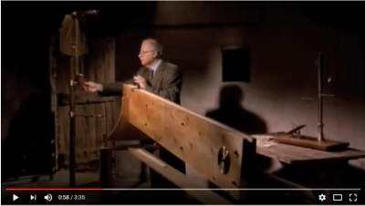
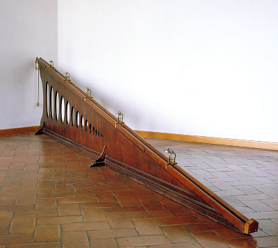
For a first project of coding using Wolfram Language I think it is hard to simulate the water clock, so I have decided to reproduce virtually the inclined plane device that can be found in the Galileo Galilei Museum of Florence. The device consists basically in a long plane equiped with little bells. I used this device myself three years ago (2014) in a trip to Florence. As it can be read in the documentation of the museum:
No documents survive proving that Galileo performed this specific experiment. In the mid-nineteenth century, Giuseppe Bezzuolifollowing the instructions of Vincenzio Antinori, director of the Museo di Fisica e Storia Naturalerepresented in a fresco of the Tribuna di Galileo the Pisan scientist conducting an experiment to demonstrate the law of falling bodies by means of an inclined plane.
This is the device that I have coded for the present project at the WSS17. The code is divided in two parts. On the first part I define the constants, variables and functions that will be used into the second part:
Part 1: Defining the functions.
(*DEFINITION OF FUNCTIONS *)
ClearAll[angle,t,g,b1,b2,b3]

(*This function draws an inclined plane of variable inclination with a ball*)
inclinedPlane[angle_, t_, g_, b1_, b2_, b3_]:=

DynamicModule[
    {\[Theta], lengthPlane,heightPlane, h, dFall, yFall, xFall, timeFall, \[Phi], ballRadius, ballCenter, ballPoint, lineBells, bellOne, t3, bellTwo, t2, bellThree, t1, bellEnd, tf},
    \[Theta] = angle * \[Pi]/180;(*inclination angle of the plane in radians*)
    lengthPlane = 400;
    heightPlane = lengthPlane * Sin[\[Theta]]; (*height of the plane*)
    h = lengthPlane * Sin[\[Theta]]+2*ballRadius*Cos[\[Theta]]; (*height of the line of bells*)
    dFall = 1/2*g*Sin[\[Theta]]*t^2;(*distance falling on the plane*)
    yFall = -dFall*Sin[\[Theta]];(*vertical distance of falling*)
    xFall = dFall*Cos[\[Theta]];(*horitzontal distance of falling*)
    ballRadius=10;
    \[Phi] = dFall/ballRadius;(*angle rotating by the ball rolling down the plane*)
    ballCenter ={ballRadius*Sin[\[Theta]]+xFall, heightPlane+ballRadius*Cos[\[Theta]]+yFall};
    ballPoint = ballCenter + {ballRadius*Sin[\[Theta]],ballRadius*Cos[\[Theta]]};
    lineBells = {{2*ballRadius*Sin[\[Theta]],lengthPlane*Sin[\[Theta]]+2*ballRadius*Cos[\[Theta]]},{lengthPlane*Cos[\[Theta]]+2*ballRadius*Sin[\[Theta]],2*ballRadius*Cos[\[Theta]]}};
    bellEnd = pointLine[1,lineBells]; (*point location of the last fixed bell*)
    bellOne = pointLine[b1,lineBells]; (*point location of the first mobile bell*)
    bellTwo = pointLine[b2,lineBells]; (*point location of the second mobile bell*)
    bellThree = pointLine[b3,lineBells]; (*point location of the third mobile bell*)
    t1 = Round[Sqrt[2*(h - bellThree[[2]])/(g*(Sin[\[Theta]])^2)],0.1];(*time of first collision ball-bell*)
    t2 = Round[Sqrt[2*(h - bellTwo[[2]])/(g*(Sin[\[Theta]])^2)],0.1];(*final of the second collision ball-bell*)
    t3 = Round[Sqrt[2*(h - bellOne[[2]])/(g*(Sin[\[Theta]])^2)],0.1];(*time of the third collision ball-bell*)
    tf = Round[Sqrt[2*(lengthPlane-ballRadius)/(g*Sin[\[Theta]])],0.1];(*final time of falling on an inclined Plane*)
    bells = {0,b3,b2,b1,1};(*is a global list variable that store the position of the balls as a ratio of lengthplane*)
    timeBells = {0,t1,t2,t3,tf};(*is a global list variable that store all the times of collisions ball-bell*)
    DynamicWrapper[
    Graphics[
       {
       (*draws the plane*)
       Style[Line[{{0,lengthPlane*Sin[\[Theta]]},{lengthPlane*Cos[\[Theta]],0}}],Blue,Thick],

       (*draws the ball*)
       Style[Circle[ballCenter,ballRadius],Red,Thick] ,

       (*draws ballPoint*)
       {PointSize[Large],Red,Point[ballPoint]},

       (*draws the final stop mark on the plane *)
       Style[Line[{{lengthPlane*Cos[\[Theta]],0},{lengthPlane*Cos[\[Theta]]+2*ballRadius*Sin[\[Theta]],2*ballRadius*Cos[\[Theta]]}}],Blue,Thick],

       (*draws the line for the bells *)
       Line[lineBells],

       (*draws the bells *)
       PointSize[Large],
       Point[bellEnd], (*point location of the last fixed bell*)
       Point[bellOne], (*point location of the first mobile bell*)
       Point[bellTwo], (*point location of the second mobile bell*)
       Point[bellThree], (*point location of the third mobile bell*)


       (*draws the radius of the ball*)
       Style[Line[{ballCenter,ballCenter+ballRadius*{-Sin[\[Theta]+\[Phi]],-Cos[\[Theta]+\[Phi]]}}],Red],

       (*draws the inclination arc of the plane*)
       Style[Circle[{lengthPlane*Cos[\[Theta]],0},100,{\[Pi]-\[Theta],\[Pi]}],Blue]
       },
    (*plot the labels*)
    PlotLabel->Style[Row[
                 {
                 "\[Theta] = ",angle,"\[Degree]",
                 "  a = ",Round[g* Sin[\[Theta]],0.1]," m/",Superscript["s",2],
                 "  t = ",Round[t,0.1],
                 " t1 = ",t1,
                 " t2 = ",t2,
                 " t3 = ",t3,
                 " tf = ",tf
                 }
                 ],
                 Black,"Label",10],
    PlotRange->{{0,400},{0,300}},
    ImageSize->425,
    Frame->True
    ],

    (*emits sound when the ball touch the bells*)
    If[

       t1 - 0.1 < Round[t,0.01]< t1 + 0.1 ,
       EmitSound[Sound[SoundNote[]]],
         If [

         t2 - 0.1 < Round[t,0.01]< t2 + 0.1 ,
         EmitSound[Sound[SoundNote[]]],
          If[

          t3 - 0.1 < Round[t,0.01]< t3 + 0.1 ,
          EmitSound[Sound[SoundNote[]]],
              If[
                 tf - 0.2 < Round[t,0.01]  ,
                 EmitSound[Sound[SoundNote[]]]
              ]
          ]
         ]
       ]
    ]
];

(*This function locate a bell on the line of bells*)
ClearAll[bell,lines]
pointLine[bell_,lines_]:=
Module[{pointLine,startPoint,finalPoint,direction},
    startPoint = lines[[1]];
    finalPoint = lines[[2]];
    direction = finalPoint - startPoint;
    pointLine = startPoint + bell*direction
    ];


(*This function compute the final time of falling on an inclined Plane*)
ClearAll[angle,lengthPlane,g]
timeFall[angle_,lengthPlane_,g_]:=
Module[{\[Theta],finalTime,ballRadius},
    \[Theta] = angle * \[Pi]/180;
    ballRadius = 10;
    finalTime = Sqrt[2*(lengthPlane-ballRadius)/(g*Sin[\[Theta]])]
    ];

(*This function map a list of Solar planets taking its gravity and and its images*)
ClearAll[planets]
menuPlanet[planets_]:=
Module[{menuSolar},
       menuSolar = Map[QuantityMagnitude[UnitConvert[#["Gravity"],"SI"]]-> Row[{#,#["Image"]}]&,planets]
    ]
Part 2: Framing the dynamic visualization with Manipulate.
Manipulate[

 inclinedPlane[angle, t, g, b1, b2, b3],

 (*configuration of controls*)
    (*the angle is measured in degrees*)
    {{angle, 5, "slope \[Theta]"}, 5, 45, 5, ControlType -> Slider} ,

    (*the position of the intermediate bells between the start and the \
end of the plane*)
    {{b1, 0, "bell 1"}, 0, 1, 0.01, ControlType -> Automatic},
    {{b2, 0, "bell 2"}, 0, b1, 0.01, ControlType -> Automatic},
    {{b3, 0, "bell 3"}, 0, b2, 0.01, ControlType -> Automatic},


    (*the time is in seconds*)
    {{t, 0.001, "release ball"}, 0.001, timeFall[angle, 400, g], 0.001,
  Trigger, AnimationRate -> 1, Appearance -> "Labeled",
  ControlPlacement -> Left},

    (*gravitational constant of Solar system planets*)
    {{g, 9.8`3., "Planet:"}, menuPlanet[PlanetData[]]},
 ControlType -> PopupMenu,


    SaveDefinitions -> True,
    ControlPlacement -> Left
 ]
Part 3: The virtual plane in any planet of the Solar system.
As a result of the code we obtain a Manipulate[] frame with:
- slide controls for the slope and the locations of the bells.
- a pop-up menu for selecting the planet of experimentation.
- a trigger button of time for releasing the ball falling down the plane (really is not a rotating ball but a sliding ball)
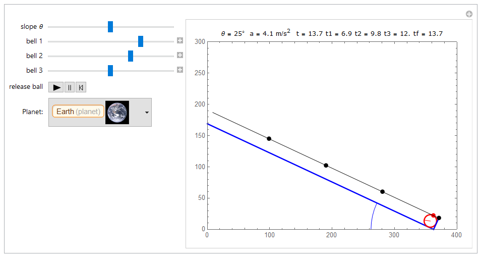
The educational purpose working with this virtual lab is that students can experiment different slopes and different positions of the bells registering the data of the respective times of falling.
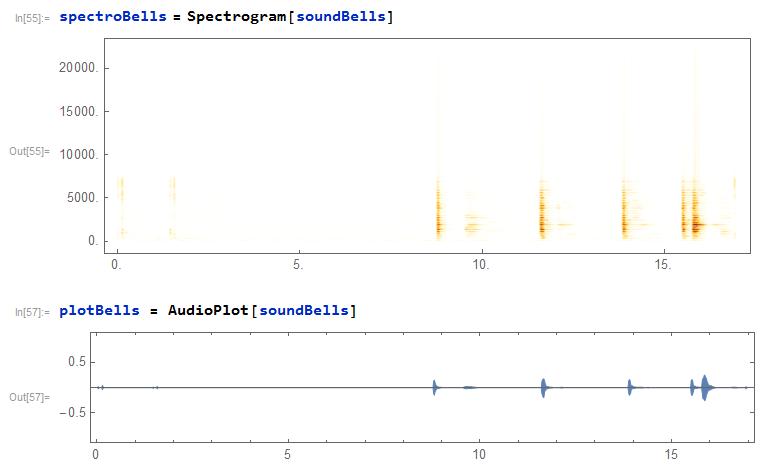
If the values of accelerations and partial times of falling are hided in the Manipulate[] frame then we can do another kind of experimentation with the student. For example, the sound of the bells can be captured and saved in a audio file inside the same notebook. After that, analyzing this audio file with an spectrogram or an audioplot the events of collision ball-bell can be deduced:
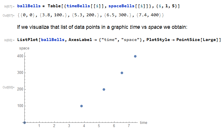
With this information, we can plot and try to fit a function for the experimental data:
distance = Interpolation[ballBells]
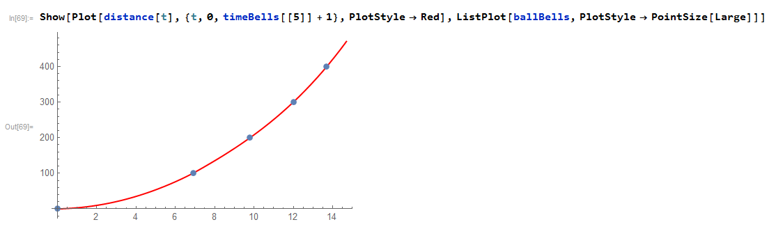
And now, with the function interpolated it is easy to construct a map of distance values for different increasing values of time between the range of time interpolated data:
dt = Map[distance, {1, 2, 4}]
It can be seen that when the time is doubled the traveled space is not doubled. On the other side it can be also seen that for equal intervals of time the distances are not increasing equally
dt = Map[distance, {1, 2, 3, 4, 5, 6, 7}]
Or we can try to interpolate a polynomial functions that fit the experimental points:
InterpolatingPolynomial[ballBells, t]
And that give to us approximately the equation of motion on the plane space[ t ] . Now we can try to answer a lot of questions with the students, as for example:
- .- What does the mathematical expression space[t] really means?
- .- If there are in the polynomial expressions of space[t], how should we interpret the cubic and quartic terms? and the first order term in t?
- .- What happens if we interpolate the experimental points only to first order? And second order?
- .- Which is now the best fitting interpolating function for our list of experimental points?
- .- What happens if the slope of the plane is changed? and if the planet is changed?
- .- Can we deduce the value of the gravity of the planet listening the sounds of the bells? How could we do that?
- .- What piece of code would we need for this goal?
- .- What if we constructed physically a real inclined plane with bells and we register the sound of the bells?
- .- How can we analyze with code the results of the real experiment?
Part 4: Conclusions.
When I started this project in the WSS17 my background on Wolfram Language was zero, so I started only knowing some aspects of the specific syntax and the structure of the coding language. Without doubt, this project has been an intensive, hard and effective way to learn WL, with a lot problems to combine the dynamic graphic with modules inside Manipulate and at the same time coding the collision events of sound. To conclude, the main difficulty remains on modelling with accuracy physic experiments in a virtual lab.
After the WSS17 experience, in the near future I would like to design new physic experiments with mechanical devices to model them using Wolfram Language and to share them in the Demonstration Project.
GitHub repository of the project
https://github.com/mcanosan/WSS2017
References
Galilei, Galileo (1638): Dialog Concerning Two New Sciences (translated by Henry Crew and Alfonso de Salvio, Macmillan 1914). Mac Douglas, D.W. (2012): Newton's Gravity. An introductory guide of the mechanics of the Universe. Catalogue Galileo Galilei Museum: http://catalogue.museogalileo.it/object/InclinedPlane.html
Wikipedia.
Wolfram MathWorld.
Wolfram Demonstration Project


