Wolfram Summer School 2017 Project
Development of a Book on Signals and Systems
Project description
The aim of this project is to start editing a new textbook on "Signals and Systems" in addition to an online ebook version with animated and dynamic illustrations using the Wolfram platform. This ebook version can be opened offline using the free Wolfram CDF player. In addition, notebook tools (palettes and DockCells) will be developed in order to make editing such a book and others easier for all Wolfram Notebook users.
Book Project - Github Repository
Please find hereafter, a sample Section of the Book.
Nyquist-Shannon Sampling Theorem
The Nyquist-Shannon Sampling theorem is a fundamental one providing the condition on the sampling frequency of a band-width limited continuous-time signal in order to be able to reconstruct it perfectly from its discrete-time (sampled) version. It stated that the sampling frequency must be at least two times the highest frequency of the continuous-time signal spectrum.
What is a Signal?
A signal is a time/space varying function which includes some useful information. Most of signals are continuous-time ones and hence can not be either stored (or transmitted) over realistic limited data storage (or band-limited propagation space) due to infinity of points to be processed. Such signals could be of different sources or types, such as audio ones, or any real life physical measure or parameter retrieved by sensors (temp, humidity, speed, ...).
    weatherData =
      WeatherData[{33.9716, 6.8498},
       "MeanTemperature", {{2016, 1, 1}, {2016, 12, 31}, "Day"}];
    DateListPlot[weatherData, Joined -> True]
- Example of a continuous-time* signal - Mean Temperature during 2016 in Rabat, Morocco:
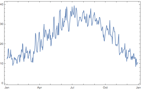
* The signal looks continuous on the plot but any signal processed (transmitted, stored or displayed) on a computer or any digital system, is always a sampled version of the original continuous time signal
In order, to process real life signals either to store or transmit, we need to a sampling process them, making them discrete-time signal.
Sampling Theorem
Sampling a continuous-time signal is getting one sample each sampling period $T_s[s]$ , which means a sampling frequency equivalent to $f_s=\frac{1}{T_s}[\text{Hz}]$.
The mean important decision to make is the sampling frequency value of $f_s$: Indeed, if its value is too big, we'll get $f_s$ samples per second, so large storage or large band width in order to transmit the data. If on the other hand, the value is too small, we won't be able to reconstruct the signal from the samples.
Hence, there is a tradeoff to make in order to minimise the needed resources (storage or frequency band-width) while being able to reproduce the original signal from the samples. One theorem provides an answer to this question, it's the Nyquist-Shannon Sampling Theorem which states:
A continuous-time signal $x(t)$ can be sampled at a frequency $fs$ in order to get a discrete-time copy of it $x[n]$ , and afterwards be reconstructed perfectly to its original form $x(t)$ if with $f_{\max }$ is the maximum frequency value of the $x(t)$ signal spectrum.
Next, we'll consider a $Sinc^2$ function and see what happen to the sampled signal on the frequency domain using Fourier Transform
Sampling Process
Time Domain Analysis
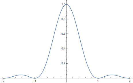
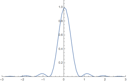
Consider the function $x(t)=Sinc^2(t)$ which represent a continuous-time signal.
x[t_] := (Sinc[Pi*t])^2;
Plot[x[t], {t, -2, 2}]
- Plot of the signal x(t)=Sinc^2(t):
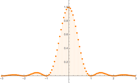
Consider a sampling frequency $f_s$ and let see what happen for different values of $f_s$.
Manipulate[
Show[DiscretePlot[x[t], {t, -3, 3, 1/fs},
PlotRange -> {{-3, 3}, {-0.1, 1.1}}, PerformanceGoal -> "Quality",
PlotStyle -> Directive[Orange, Thick], PlotMarkers -> Automatic],
Plot[x[t], {t, -3, 3}]], {{fs, 15.25, "Frequency Subscript[f, s]"}, 0.5, 30, Appearance -> "Labeled"}, SaveDefinitions -> True]
- Plot of the continuous-time and discrete-time (sampled) signals:
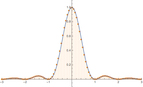
As we can see, for high values of $f_s$ we can at least recognize visually the original continuous-time form on the $x(t)$ signal. However, for small values of $fs$ such as $f_s=0.1$ hz for instance, we can no more visually retrieve the form of the original $Sinc^2$ function, with only four sample over the $20$ interval duration it's quite impossible to go back from samples to continuous signal. Indeed, in such case, we are sure not satisfying the Nyquist-Shannon sampling condition. In the time domain, we can somehow visually understand what's happening, however, the theorem is more understandable when analyzed on the frequency domain.
Frequency Domain Analysis
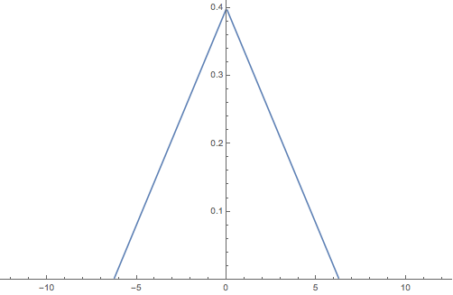
The spectrum analysis of signal $x(t)$ allows us to understand easily and even prove the theorem ourselves. $$\text{TF}\left(\text{Sinc}^2 (a t)\right)=\frac{1}{\left| a\right|} \text{tri}\left(\frac{t}{a}\right)$$
Fourier Transform of the signal x(t):
Simplify[FourierTransform[x[t], t, \[Omega]]]
$$\frac{-2 \omega \text{sgn}(\omega )+(\omega -2 \pi ) \text{sgn}(\omega -2 \pi )+(\omega +2 \pi ) \text{sgn}(\omega +2 \pi )}{4 \sqrt{2} \pi ^{3/2}}$$
Spectrum of the signal x(t):
Plot[FourierTransform[x[t], t, \[Omega]], {\[Omega], -10*2 Pi,
  10*2 Pi}, PlotRange -> {{-2*2 Pi, 2*2 Pi}, {0, 0.41}}]
Sampled signal xn and its Fourier transform spectrum:
Manipulate[
 Row[{DiscretePlot[x[t], {t, -3, 3, 1/fs},
    PlotRange -> {{-3, 3}, {-0.1, 1.1}}, PerformanceGoal -> "Quality",
     PlotStyle -> Directive[Orange, Thick], PlotMarkers -> Automatic,
    ImageSize -> 340],
   ListLinePlot[
    Join @@ Table[
      Abs[Fourier[Table[N[x[n/fs]], {n, -4*fs, 4*fs + 1}]]], 4],
    DataRange -> {-4 Pi, 4 Pi},
    PlotRange -> {{-4 Pi, 4 Pi}, {0, 1.5}}, ImageSize -> 300]}], {{fs,
    15.25, "Frequency Subscript[f, s]"}, 0.5, 20, Appearance -> "Labeled"}]
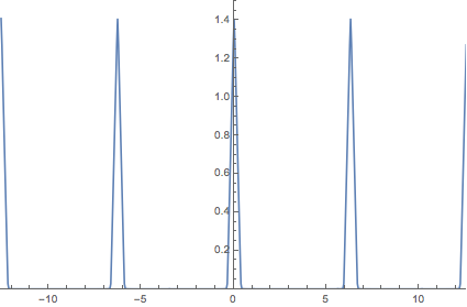
The spectrum of the sampled signal is a periodic form where it's period is $2\pi$, and as long as we respect the Nyquist-Shannon condition, its form over one period is equivalent to the spectrum of the original continuous-time signal $x(t)$. Indeed, while the sampling frequency $fs$ is large enough, there is no overlapping between the periods of the spectrum, and then, the original signal can be retrieved by mean of a low passband filter. However, if the sampling frequency is too low, such as $fs\leq 1.4$ in the above example, there will be overlapping of the spectrum, which we call an aliasing effect. In such a case, we can no more retrieve the original signal using a simple low-passband filter, and we need then a more powerful signal processing by means of equalization. The condition to avoid the overlapping is that $fs > 2 f_\max$, which represents perfectly the Nyquist-Shannon sampling theorem.
Reconstruction Process
The reconstruction process consists in the generation of the original continuous-time signal $x(t)$ from the sampled version $x[n]$. As long as there is no aliasing effect, a simple low passband filter is enough to retrieve the original signal
Filtering the Spectrum of the sampled signal x[n]:
Manipulate[
 Show[ListLinePlot[
   Join @@ Table[Abs[Fourier[Table[N[x[n/fs]], {n, -4*fs, 4*fs}]]],
     2], DataRange -> {-2 Pi, 2 Pi},
   PlotRange -> {{-2 Pi, 2 Pi}, {0, 1.5}}, ImageSize -> 300],
  Plot[HeavisidePi[x/(2*Pi)], {x, -2 Pi, 2 Pi}, Exclusions -> None,
   PlotStyle -> Directive[Orange, Thick, Dashed] ]], {{fs, 8,
   "Frequency Subscript[f, s]"}, 0.5, 20, Appearance -> "Labeled"}]
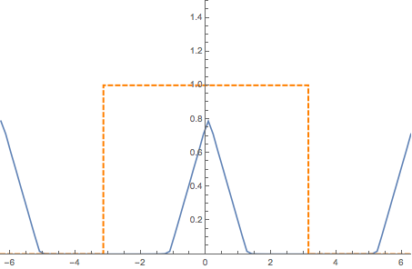
Depending on the existence of aliasing or not, the retrieved continuous-time signal could the perfect copy of the original or a distorted one.
Spectrum of the sample signal and the reconstructed version of the signal x[n]:
Manipulate[
 Row[{Show[
    ListLinePlot[
     Join @@ Table[Abs[Fourier[Table[N[x[n/fs]], {n, -4 fs, 4 fs}]]],
       2], PerformanceGoal -> "Quality", DataRange -> {-2 Pi, 2 Pi},
     PlotRange -> {{-2 Pi, 2 Pi}, {0, 1.5}}, ImageSize -> 300],
    Plot[HeavisidePi[x/(2*Pi)], {x, -2 Pi, 2 Pi}, Exclusions -> None,
     PlotStyle -> Directive[Orange, Thick, Dashed] ]],
   ListLinePlot[
    Re[InverseFourier[Fourier[Table[N[x[n/fs]], {n, -4 fs, 4 fs}]]]],
    DataRange -> {-3, 3}, PlotRange -> {{-3, 3}, {0, 1.1}},
    ImageSize -> 300, PerformanceGoal -> "Quality"] }], {{fs, 8,
   "Frequency Subscript[f, s]"}, 0.5, 20, Appearance -> "Labeled"}]
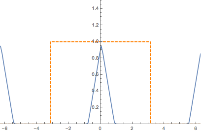
As long as the sampling frequency verifies the Nyquist-Shannon condition, we can reconstruct the original signal without distortion.