The goal: to make an unique LHC data easier accessible and understandable, aiming to help all interested to perform the experimental data analysis.

Large Hadron Collider (LHC) the largest world known particle accelerator with achieved collision energy for now of 13 TeV. It was designed to be the most powerful machine to study the fundamental physics. To record the proton-proton collisions happens at the LHC four huge detectors were constructed, namely: ATLAS, CMS, LHCb and ALICE. In 2016 at CERN the experimental data was released to the public community and could be find at the Open Data Portal: http://opendata.cern.ch

In current work the first steps in the extracting data, recorded by the CMS detector, and analyzing it in Mathematica are presented.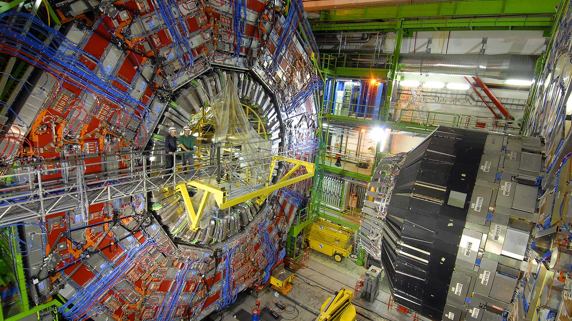

The data sample extraction was done in two steps: 1) using CMS open software to select the sample from the primary datasets; 2) using Mathematica to import the data from reduced root files and text files. (more details on the data extraction from the ROOT format see the notebook file here )

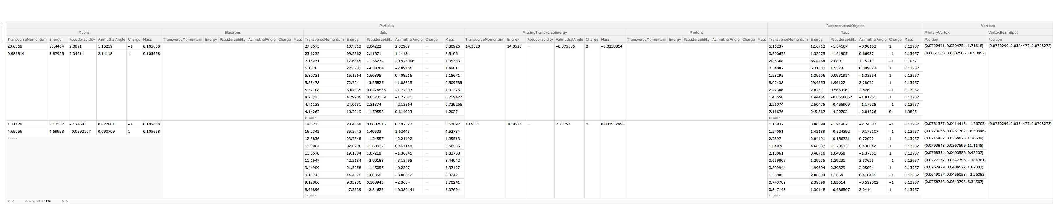
The imported data has a structure readable by Mathematica and does not required previous knowledges about experimental software, in order to analyze it.

In order to reject events that does not pass analysis criteria, the cut function was implemented.

applyCut[object_, type_, filter_, n_ , operator_][event_] := 
 operator[Length[Select[event[[object, type]], filter]], n]

For example: to select an event with exactly one muon which has transverse momentum greater than 20 GeV and pseudorapidity less than 2,1.

datasetOneMuon = 
 dataset[Select[applyCut["Particles", "Muons", True &, 1, Equal]]]

datasetMuonCuts = 
 datasetOneMuon[
  Select[applyCut["Particles", 
    "Muons", #TransverseMomentum > 20 && Abs[#Pseudorapidity] < 2.1 &,
     1, Equal]]]

The functionality for calculation of the kinematic variables relevant for the analysis are also presented here:

energyFormula[particle_] := 
 Sqrt[(particle["TransverseMomentum"]*
      Cosh[particle["Pseudorapidity"]])^2 + particle["Mass"]^2]

pXFormula[particle_] := 
 particle["TransverseMomentum"] * Cos[particle["AzimuthalAngle"]]

pYFormula[particle_] :=  
 particle["TransverseMomentum"] * Sin[particle["AzimuthalAngle"]]

pZFormula[particle_] := 
 particle["TransverseMomentum"] * Sinh[particle["Pseudorapidity"]]

For example we could show the x component of the momentum of all Jets: Histogram[pX[All, "Particles", "Jets", All], {0.5}]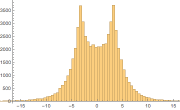

Particle three and four-momentum:

threeMomentumFormula [particle_] := {pXFormula[particle], 
  pYFormula[particle], pZFormula[particle]}

fourMomentumFormula[particle_] := {energyFormula[particle], 
  pXFormula[particle], pYFormula[particle], pZFormula[particle]}

Angular separation between particles:

deltaRFormula[particle1_, particle2_] := 
 Sqrt[(particle1["Pseudorapidity"] - 
      particle2["Pseudorapidity"])^2 + (particle1["AzimuthalAngle"] - 
      particle2["AzimuthalAngle"])^2]

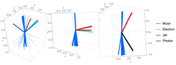
The collision events visualization functionality was carried out in this work:

momMuons = threeMomentum[nEv, "Particles", "Muons", All];
momJets = threeMomentum[nEv, "Particles", "Jets", All];
momElectrons = threeMomentum[nEv, "Particles", "Electrons", All];
momPhotons = threeMomentum[nEv, "Particles", "Photons", All];

Legended[Graphics3D[{Style[Line[{{0, 0, 0}, Normalize[#]}], Hue[.99], 
      Thickness[Log@Norm[#]/200]] & /@ momMuons, 
   Style[Line[{{0, 0, 0}, Normalize[#]}], Hue[.6], 
      Thickness[Log@Norm[#]/300]] & /@ momJets,
   Style[Line[{{0, 0, 0}, Normalize[#]}], Hue[.43], 
      Thickness[Log@Norm[#]/200]] & /@ momElectrons,
   Style[Line[{{0, 0, 0}, Normalize[#]}], 
      Thickness[Log@Norm[#]/200]] & /@ momPhotons}, Axes -> True, 
  AxesLabel -> {x, y, z} ], 
 LineLegend[{Red, Green, Blue, Black}, {"Muon", "Jets", "Electron", 
   "Photon"}]]

It is possible to read information from the root file in Mathematica as explained: http://library.wolfram.com/infocenter/Articles/7793/

Import["/Users/mac/Downloads/MyF/analyzeFWLite.root", "ROOT"]

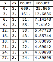
muonPy = Import[
  "/Users/mac/Downloads/MyF/analyzeFWLite.root", {"ROOT", "TH1FData", 
   "muonPy"}]

head = {"x", "\[CapitalDelta]x", "count", "\[CapitalDelta]count"};
Grid[Join[{head}, Take[muonPy, 10]], Frame -> All]

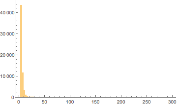
to plot the histograms from the root file:

graphics1JetPt = 
 Import["/Users/mac/Downloads/MyF/analyzeFWLite.root", {"ROOT", 
   "TH1FGraphics", "jetPt"}]

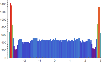
graphics2JetEta = 
 Import["/Users/mac/Downloads/MyF/analyzeFWLite.root", {"ROOT", 
   "TH1FGraphics", "jetEta"}, 
  ColorFunction -> Function[{height}, ColorData["Rainbow"][height]]]