This project was conducted during Wolfram Summer Camp 2017. As I had previously conducted research related to Greatest Common Divisors, I was able to further explore my field of interest through this opportunity.

GIF

Below is the result of this project: a 5D plot of Gaussian Integers pairs $(x,y)$ that satisfy $ 9<|gcd(x,y)| \leq 16\sqrt2$ from three different viewpoints.

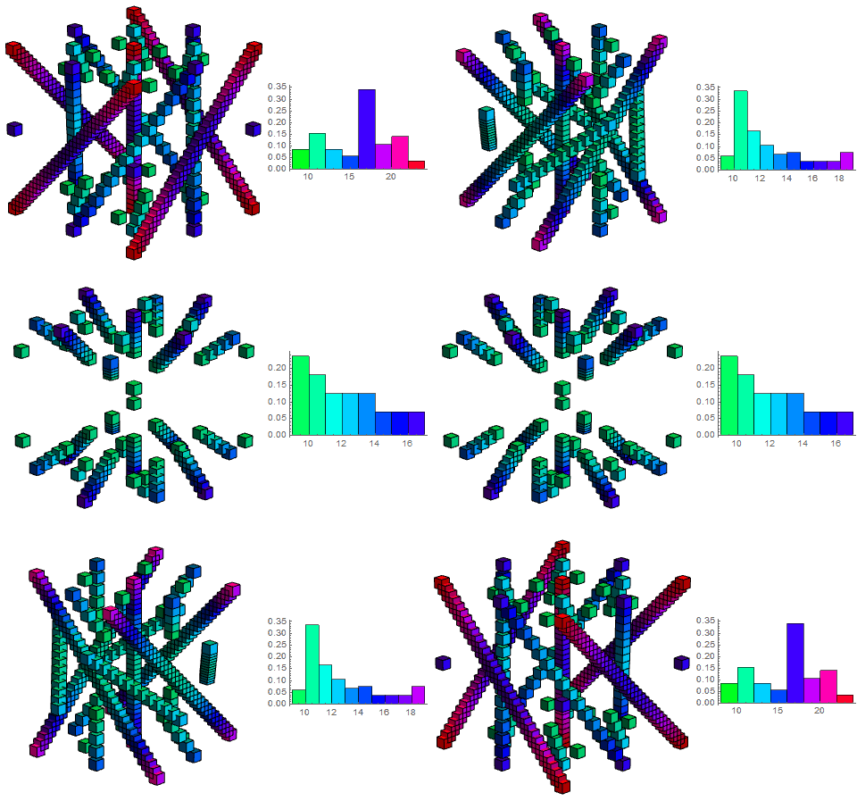Corner View 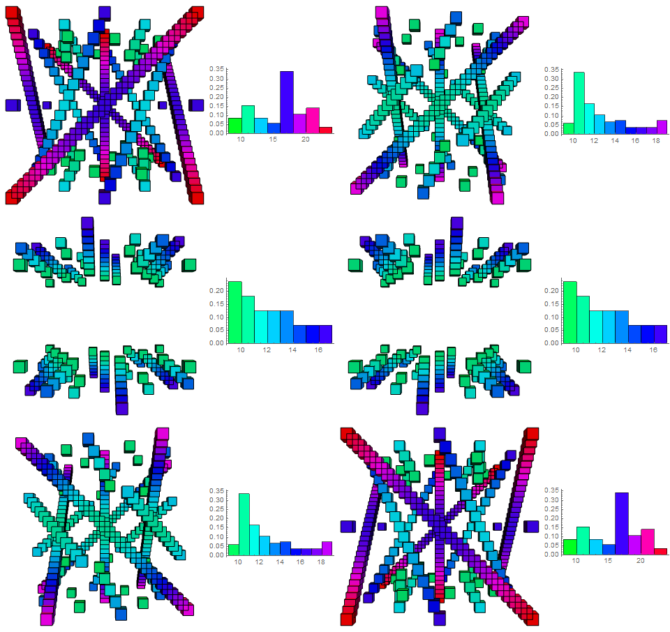Front View 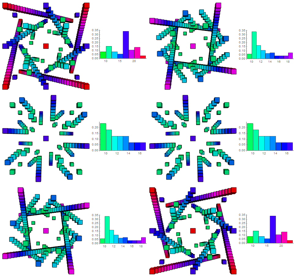Top View

Problem:

The visualization of Greatest Common Divisors of Integers is widely known. For instance, the following is a black-and-white representation of coprime pair integers. The horizontal and vertical edges represent number lines, and where they intersect is colored black if they are co-prime.

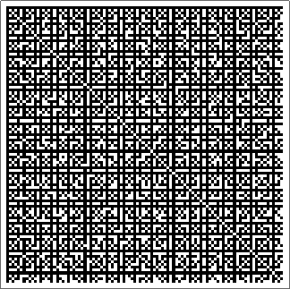ArrayPlot of Coprime Integer Pairs

Through this project, I attempt to extend the visualization from the original integers to the Gaussian number field.

We will begin with basic definitions.

Gaussian Integer: A number of the form $a+bi$, where a and b are integers. (Ex. 2+3i)

Norm of a Gaussian Integer: The norm of $a+bi$ is defined as the following. $$|a+bi|= \sqrt {a^2+b^2} $$

Greatest Common Divisor: The Gaussian Integer with the greatest norm (absolute value) that divides both numbers. (Ex. $\gcd(2, 3+3i)=1+i$)

The objective of my visualization is to represent the norm of the gcd of every pair of Gaussian Integers. This is equivalent to plotting the following function $f$.

$$f(a,b,c,d)=|gcd(a+bi, c+di)| , \quad\text{for}\;\; a,b,c,d\in \mathbb Z $$

Since there are 4 variables as input, and 1 variable as the output, I used the following methodology to plot the 5D function

Method:

Consider all Gaussian Integers $p+qi$ within the range $$ -n \leq p , q \leq n.$$ We then choose every pair of two Gaussian Integers, each given by $a+bi$ and $c+di$. The absolute value of the two integers is denoted as $e$.

1. Among the given inputs $a$, $b$, $c$, $d$, we choose $a$, $b$, $c$ and assign it to the coordinate $(a,b,c)$ in 3D space
2. We define the 4th variable $d$ with time. $d$ is assigned to step number $d+n+1$ out of a total $2n+1$ steps of the plot.
3. The output $e$ is divided by the maximum absolute value possible, $\sqrt2 n$, and is assigned to a color between red and purple by the Hue function.

Still Shot:

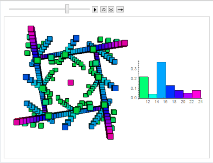
This image describes the gaussian integer pairs of the form $$ |gcd(a+bi, c+14i)|>10, \quad\text{for} \;\; -19\leq a,b,c \in \mathbb Z \leq 19$$ In other words, $d$ is 14 in this case.The histogram represents the frequency of the colors, which are equivalent to the absolute value of the GCD. For instance, light green represents a gaussian integer pair who has an absolute value of the gcd between 10 and 12.

Conclusion:

Thus, one cycle of the above GIF represents a "plot" of our 5D function. It is interesting that the animation contains both regularity (patterns consistently emerging and disappearing), and irregularity (random blocks appearing and vanishing). Although it is difficult to exactly capture what is going on within the plot, i believe it will be an interesting subject of further research.

Mathematica Code:

Below is the code for the GIFs above.

First, I chose all pairs of Gaussian integers that have a gcd with a magnitude larger than a given value, for a certain d. Then, I assigned it to a cuboid with its center at coordinate $(x,y,z)$, Afterwards, a color was assigned depending on the norm of the GCD.

DesiredPoints[n_, fourth_, length_, 
  min_] := (lis = 
   Select[Flatten[
     Table[{a, b, c}, {a, -n, n}, {b, -n, n}, {c, -n, n}], 2], 
    Abs[GCD[#[[1]] + I*#[[2]], #[[3]] + fourth*I]] > min &]; {Hue[
      Abs[GCD[#[[1]] + I*#[[2]], #[[3]] + fourth*I]]/(Sqrt[2]*n)], 
     Cuboid[# - {length, length, length}, # + {length, length, 
        length}]} & /@ lis)

Next I generated Histograms which represent the relative frequency of each color for a given value of $d$.

Histo1[n_, k_, m_] := 
 Select[Abs[GCD[#[[1]] + I*#[[2]], #[[3]] + k*I]] & /@ 
   Flatten[Table[{a, b, c}, {a, -n, n}, {b, -n, n}, {c, -n, n}], 
    2], # > m &]
Histo2[n_, fourth_, min_] := (c = Length[Histo1[n, fourth, min]]; 
  t[{{xmin_, xmax_}, {ymin_, ymax_}}, ___] := {Hue[xmin/(Sqrt[2]*n)], 
    Rectangle[{xmin, ymin/c}, {xmax, ymax/c}]}; 
  Histogram[Histo1[n, fourth, min], ChartElementFunction -> t])

The code below generates the table that can be utilized for making GIFs or Animated Lists

TableForExport[n_, min_, size_, viewpoint_] := 
 Table[Row[{Graphics3D[DesiredPoints[n, k, size, min], 
     BoxStyle -> Directive[Hue[1, 1, 1, 0]], ViewPoint -> viewpoint, 
     ImageSize -> 300], Histo2[n, k, min]}, 
   BaseStyle -> ImageSizeMultipliers -> .5], {k, -n, n, 1}]

This final code generates the actual visualizations.

ListAnimate[TableForExport[16, 9, 1, Top]]
Export["16_9_top.gif", TableForExport[16, 9, 1, Top], 
 "AnimationRepetitions" -> Infinity]