Description

In this exploration, I explored the halting times of Turing machines. A Turing machine is essentially consists of a set of rules that can be applied to successive cells on a infinitely long tape of typically blank cells. Each step in a Turing machine is characterized by the state (color) of the current cell and the direction in which the head is turned.

A set of rules for a Turing machine might resemble as follow:

This rule dictates, for example, that when the head is position 1 (up) and the cell it is on is likewise in position 1 (orange), the cell below it should become orange and the head, still facing up, should move a distance of -1 (one unit left). This can be notated as {1,1} -> {1,1,-1}.

A common issue in the study of Turing machines is the halting problem, or whether and when a Turing machine will cease moving. Generally, this problem has been proved to be incomputable. However, it is possible to determine halting probabilities for more specific cases.

I have investigated two definitions of halting in the following study. The first defines halting within the rules of a Turing machine; that is, when a Turing machine reaches a particular head-cell combination, it will halt. The second defines halting merely as a cessation of changing cell states. When a halting state is reached in this instance, the head may move as it pleases, but the resulting cell states will not differ from step to step.

Basic Points

Some basic principles to establish:

• A Turing machine can do one of three things: halt relatively quickly, never halt, or continue on for an indefinite amount of time before reaching a halt state.
  • This third instance generally pertain to Turing machines where it is not obvious that the machine will never halt. After all, in some cases the repetition of steps in a machine leaves no room for halting motion.
  • For the sake of simplicity, these three kinds of machines will be referred to as halting, non-halting, and weird Turing machines.
• A Turing machine will not halt unless some halt state is specified.
  • There will always be some rule dictating what the machine should do next that correspond to the current position of the head and cell.
  • Therefore, for a Turing machine to halt it needs some rule in some way, shape, or form that corresponds to a halt state.
• A Turing machine does not necessarily halt even if a halt state is specified.
  • For example, a machine may enter a loop here it goes through the same few steps infinitely, never achieving a halt state.
  • On the other hand, some Turing machines halt immediately; the first step they take is halting.
• Given a known maximum halting time for a specific kind of Turing machine, any machine that does not halt before the maximum time will not halt after.

Halting as Defined by Rules

As aforementioned, a Turing machine will not halt unless some halt state is specified. In this instance, the halt state for a given Turing machine was defined within the set of rules in a manner similar to busy beaver Turing machines. Busy beavers are machines with n head states and 2 cell states (denoted n, 2) which attempt to achieve the maximum amount of a given cell state before halting with known maximum halt values of 6, 24, and 107 step for 2, 3, and 4 head states, respectively. The rules can be defined by assigning every head state (s) on a cell of state (a) to a new head state (sp), cell state (ap), and head displacement (off), denoted {s, a} -> {sp, ap, off}. Here, the halt state was indicated by assigning a single {s, a} in any set of rules to {0, 3, 0}. In practice, this did not actually halt the Turing Machine, but it did provide a method to determine when a machine would have halted. As no other rule would result in a head state of zero or a cell state of three, it was easy to identify both visually and computationally which machines "halted".

The below functions describe the process for finding the probability whether and when a 2, 2 Turing machine will halt.

TM[n_, x_] :=  TuringMachine[n, {1, {{}, 0}}, x]           (* A simpler, more convenient way to write the TuringMachine function. *)
HEADS2 = Permutations[Flatten[Table[{i, j}, {i, 1, 2}, {j, 0, 1}], 1]];            (* Creates all possible head states *)
pCELLS2 = Permutations[Flatten[Table[{i, j, k}, {i, 1, 2}, {j, 0, 1}, {k,{-1, 1}}],2],{3}];   (* Creates all possible cell states *)
RuleMaker2[x_] := Table[Join[Thread[Rule[Rest[x], pCELLS2[[m]]]], {First[x] -> {0, 3, 0}}], {m,1, Length[pCELLS2]}]  (*Creates machine rules*)
Halting2 = 
  Flatten[Table[
    Select[RuleMaker2[n], ! FreeQ[TM[#, 8], {0, _, _}] &], {n, 
     HEADS2}], 
   1];            (* Lists all sets of rules that eventually halt*)
 NonHalting = 
  Flatten[Table[
    Select[RuleMaker2[n], FreeQ[TM[#, 8], {0, _, _}] &], {n, HEADS2}],
    1];     (* Lists all sets of rules that do not halt*)

N[Length[Halting2]/(Plus[Length[Halting2], 
   Length[NonHalting]])] (* Gives approximate halting probability*)

The last functions returns that any given 2,2 Turing machine with a halting state defined in its rules has about a 43.3% chance of halting.

The total amount of rules that halt at a certain step is given by the following function:

HaltStep1 = KeySort[Counts[Table[First@Flatten[Position[First /@ TM[#, 8] &@n, {0, _, _}]] - 1, {n, Halting2}]]]   
Thread[Rule[Keys[HaltStep1], Table[N[x/100] "%", {x,HaltStep1}]]]     (* The percentage of machines that halted at a certain step*)          

The -1 accounts for the initial step listed in the returned machine. The results of these functions are that:

<|1 -> 2016, 2 -> 1008, 3 -> 288, 4 -> 108, 5 -> 12, 6 -> 60|>
{1 -> 20.16 "%", 2 -> 10.08 "%", 3 -> 2.88 "%", 4 -> 1.08 "%", 5 -> 0.12 "%", 6 -> 0.6 "%"}

Corresponding list plot that plots the step at which a function halts against how many functions halt at that step:

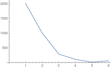
For the most part, there is a great downward trend concerning at what step a 2,2 Turing machine halts. It is far more likely for a machine to halt at the first step than at the sixth. This makes a certain amount of sense. The Turing machines that halted at the first step would have to consist of all those whose rules dictated that when the head state is 1 and the cell state is 0, halt. Any rule with this as part of its rule set will definitely halt on step 1. However, those rules that halt on step 2 had to depend on two factors: the rule dictating what should happen after the initial state, and the rule dictating what should be done after that. It would follow that this compounding complexity results in less instances of halting. And of course, each step results in more complexities, leading to less instance of halting.

However, it so happens a machine is five times more likely to halt at the sixth step than at the fifth. This may be a quirk of 2,2 Turin machines, I suppose, or it may be that at a certain point complexities begin to cancel out. If this is the case, then it would be something like mixing up a Rubik's cube. You can only mix up the pieces to a certain degree; after that, some moves begin to solve it, if even a little. It would seem that the increasing complexity is counteracted enough by this effect in order to produce more halting Turing machines than expected.

Furthermore, although the curve is relatively smooth, no function approximates it quite that well.

FindFormula[List @@ HaltStep1];
 Plot[1128.` + 3291.8` #1 - 3435.5` #1^2.` + 1204.` #1^3.` -182.5` #1^4.` + 10.2` #1^5.` &@x, {x, 0, 7}]

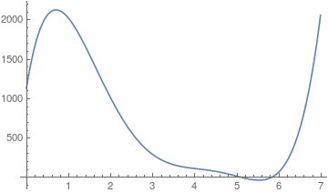
Theoretically, the above process could be performed for 2,3 and 2,4 Turing machines as well. However, the run time to Halting3 (the 2,3 machine counterpart to Halting2) was taking so long so as to be incompatible with my time constraints, and it could be imagined that functions dealing with 2,4 machines would take even longer.

An example of functions that could potentially produce results if run:

HEADS3 = Permutations[Flatten[Table[{i, j}, {i, 1, 3}, {j, 0, 1}], 1]];
pCELLS3 = 
  Permutations[
   Flatten[Table[{i, j, k}, {i, 1, 3}, {j, 0, 1}, {k, {-1, 1}}], 
    2], {5}];
RuleMaker3[x_] := 
 Table[Join[
   Thread[Rule[Rest[x], pCELLS3[[m]]]], {First[x] -> {0, 3, 0}}], {m, 
   1, Length[pCELLS3]}]
Halting3 = 
  Flatten[Table[
    Select[RuleMaker3[
      Part[HEADS3, RandomInteger[720]]], ! 
       FreeQ[TM[#, 26], {0, _, _}] &], 10], 1];

Overall, the function FreeQ[TM[n_List, x_],{0,_,_}]&] can be used on a single Turing machine with a halting state defined in its rules in order to determine whether it will halt.

Halting as Defined by Cell State

An alternative way to define a halting state could be to claim the machine halts when the cell state no longer changes from step to step. This, however, allows for the head to keep changing position. To check to see whether this happens in a Turing machine without a halt state explicitly defined in its rules, I created a function that looks for three repeats in a row at x-1, x, and x+1 steps, then checked to see whether this pattern held true at 2x. Originally, I had not thought to check the pattern at 2x, as it seemed natural to me that a Turing machine that produces the same result three times in a row would continue to do so for the fourth, fifth, sixth, etc. time. However, I had discounted the fact that the head moves and may be in different positions even when cell states are identical, leading to a mistake in computations that I caught when I plotted the halt times of various Turing machines and discovered surprising outliers that could only be accounted for by the fact that they don't actually halt.

In the following incorrect Plot, older and incorrect versions of RepeatingBoolean and HaltWhen are being used. These will be defined correctly later. RepeatingBoolean returns True if a function repeats and therefore halts at a point, and HaltWhen checks at what point the repeating state first occurs, indicating the halt state.

ListPlot[Counts[Table[Module[{x = RandomInteger[4095]}, If[RepeatingBoolean[x, 100], HaltWhen[x, 100]]], 1000]]]

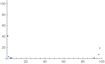
Note how most Turing machines had halted, as expected, between 0 and 5 steps. Some machines, however, appeared to halt close to the 100th step when in fact they merely had three identical cell states at that point.

The proper way to follow through with this process goes as follow:

RepeatingTM[rule_, n_] := If[Apply[SameQ, Last /@ Part[#, {n - 1, n, n + 1, 2 n}] &@TM[#, 2 n] &@
    rule], {rule, "Halts"}, {rule, "Doesn't Halt"}] 
(*Takes a rule and the number of steps the rule should run and returns whether a given rule halts or not*)

HaltWhen[rule_, n_] := First@First@Position[TM[rule, 2 n], Last@Part[TM[rule, 2 n], 2 n]] - 1  
(* Shows at what step a function halts.*) 

The -1 in the above function accounts for the fact that some Turing machines may "halt" from their initial position: they never changed from their initial state, and halt at step 0. Here n should represent the same n used in RepeatingTM, as it might not necessarily work if a smaller value is chosen. Although this function will produce a result for a non-halting function, it shouldn't be used for that purpose.

ProbabilityTM[h_, k_] := 
 N[Mean[#]/1000] &@
  Table[Length[
    Select[Table[
      RepeatingTM[{RandomInteger[(2 h k)^(h k) - 1], h, k}, 100], 
      1000], ! FreeQ[#, {_, "Halts"}] &]], 20]

This function takes h to be amount of head states of a machine and k to be the amount of cell states in a Turing machine. It then generates 1000 random Turing machines (where the rule is represented as a number between 0 to ((2 h k)^(h k)-1), the total amount of possible h,k Turing machines) and checks after 100 steps whether it halts or not. This should be sufficient for most machines.

Using the above function, one can generate a table of probabilities for Turing machines ranging from having 2 head and 2 cell states to those having 6 head and 6 cell states.

ProbabilityTable = Table[ProbabilityTM[i, j], {i, 2, 6}, {j, 2, 6}]; 
Grid[Join[{{"h\c", 2, 3, 4, 5, 6}}, Table[Prepend[Part[ProbabilityTable, k - 1], k], {k, 2, 6}]], Frame -> All] 

![enter image description here][5]

In the above grid, the "h" column represents the amount of head states of a Turing machine while the "c" row represents the cell states. (The error indicated on the right side of the cell only occurs because \c is "an unknown string escape". As I am using the notation h\c only to more clearly label the grid, this error is inconsequential.)

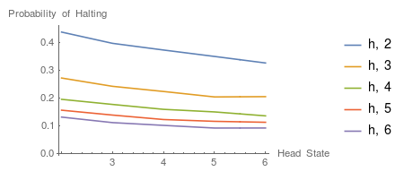
This data can be used to observe trends both when the cell states keep constant while the head states change and when the head states are constant and the cell state changes.

(* Cell states constant, head states change*)
ListLinePlot[ 
 Table[{i + 1, Part[#, j] &@Part[ProbabilityTable, i]}, {j, 1, 5}, {i,
    1, 5}], PlotLegends -> {"h, 2", "h, 3", "h, 4", "h, 5", "h, 6"}, 
 AxesLabel -> { "Head State", "Probability of Halting"}]

(* Head states constant, cell states change*)
ListLinePlot[ 
 Table[{i + 1, Part[#, i] &@Part[ProbabilityTable, j]}, {j, 1, 5}, {i,
    1, 5}], PlotLegends -> {"2, c", "3, c", "4, c", "5, c", "6, c"}, 
 AxesLabel -> { "Cell State", "Probability of Halting"}]

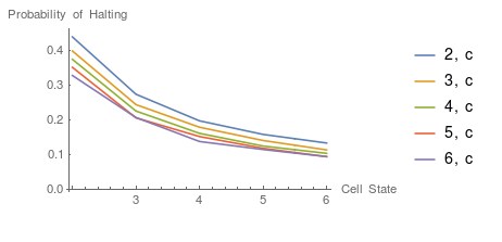
The cell state appears to determine halting probabilities to a greater degree than cell state. This makes sense, as per this definition of halting it was cell state, not head state, that determined when a machine should stop. In that respect it must be that head state alters halting probability only by increasing the complexity of the machine. As described in context with Halting1, an increase in complexity gives more possible states for a machine to be in, though the amount of those states that result in halting may not increase.

Although it is possible to find functions that somewhat resemble the above plots, for the most part approximations are still inaccurate.

Constant Cell States:

FindFormula /@ 
  Table[{i + 1, Part[#, j] &@Part[ProbabilityTable, i]}, {j, 1, 
    5}, {i, 1, 5}];
Table[Plot[Part[%24, k]@x, {x, 0, 7}], {k, 1, 5}]

Constant Head States:

FindFormula /@ 
  Table[{i + 1, Part[#, i] &@Part[ProbabilityTable, j]}, {j, 1, 
    5}, {i, 1, 5}];
Table[Plot[Part[%26, k]@x, {x, 0, 7}], {k, 1, 5}]

The below function randomly selects 2,2 Turing machines and detects when those that halt do so.

RepeatingBoolean[rule_, n_] := Apply[SameQ, Last /@ Part[#, {n - 1, n, n + 1, 2 n}] &@TM[#, 2 n] &@rule]        
 (* Returns TRUE when a machine halts and FALSE when it doesn't *)
HaltStep22 = 
 KeySort[Merge[{Counts[
     Table[If[RepeatingBoolean[x, 100], HaltWhen[x, 100]], {x, 0, 
       4095}]], <|3 -> 0|>}, Total]]
Thread[Rule[Keys[Drop[HaltStep22, -1]], 
  Table[N[100 x/Plus @@ Values[Drop[HaltStep22, -1]]] "%", {x, 
    Values[Drop[HaltStep22, -1]]}]]]

This returns:

<|0 -> 1568, 1 -> 178, 2 -> 20, 3 -> 0, 4 -> 6, 5 -> 2, Null -> 2322|>
{0 -> 88.3878 "%", 1 -> 10.0338 "%", 2 -> 1.1274 "%", 3 -> 0., 4 -> 0.338219 "%", 5 -> 0.11274 "%"}

Corresponding list plot:

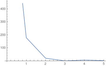
Although the halt times for HaltStep1 ranged from 1 to 6, the halt times for HaltStep22 ranged from 0 to 5. This arises mainly through the different definitions of "halting" in each case. For example, it would clearly be impossible for a machine to halt after 0 steps using the first definition; that would mean that it halted before it even started. This, however, is acceptable per the second definition, as this definition describes a change in state rather than a state in itself. That is, when there is no change in state, the machine is said to halt, as opposed to reaching a single "halt state". Furthermore, it appears that HaltStep22 never halts at 6 or 3 steps. This may be a random consequence; the low amount of machines that halt at 4 and 5 steps would certainly allow it. However, it is interesting how both in HaltStep1 and HaltStep22 briefly increase after a stretch of decreasing values. Perhaps this corresponds with the aforementioned "canceling out", but more data is needed for a complete conclusion.

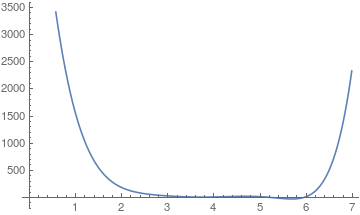
As with HaltStep1, no function quite approximates this trend.

FindFormula[List @@ HaltStep22]
Plot[8659.05 - 12756.8 #1 + 7595.42 #1^2 - 2199.33 #1^3 + 265.796 #1^4 + 8.55533 #1^5 - 5.07196 #1^6 + 0.339872 #1^7 &@x, {x, 0, 7}]

Comparing the results of the first definition of halting with the second, it can be noticed that although neither exceed six steps to halt, with HaltStep22 it is generally more likely that the machine will halt at or before the first step.

{PieChart[Values[HaltStep1], ChartLabels -> Keys[HaltStep1]], 
 PieChart[ Drop[Values[HaltStep22], -1], 
  ChartLabels -> 
   Placed[Keys[HaltStep22], 
    "RadialOuter"]]}
(* Left pie chart represents HaltStep1, right HaltStep2 without the Null values*)

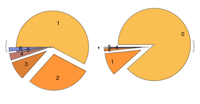
The following chart further emphasizes how much more likely it is for a function to halt at 1, compared to other values, in Halting22.

PieChart[ Take[Values[HaltStep22], 2 ;; 6], ChartLabels -> Placed[{1, 2, 3, 4, 5}, "RadialOuter"]]

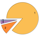
Much like with the computing issue of Halting1, it is difficult to garner complete information about the halting patterns of higher order Turing machines with this method. Although it is easier to select Turing machines at random, there are substantially more Turing machines to choose from, which requires a larger sample size to accurately depict probabilities. In fact, as there are 2985983 machines of the 2,3 degree, (compared to the 4095 of the 2,2 degree), even 100,000 randomly selected machines may not produce a significant percentage of halting machines.

Halt23 =  
 KeySort[Counts[
   Module[{x = RandomInteger[2985983]}, 
    Table[If[RepeatingBoolean[{x, 2, 3}, 100], 
      HaltWhen[{x, 2, 3}, 100], "NONHALTING"], 100000]]]]

This usually returns <|"NONHALTING" -> 100000|>.

Weird Turing Machines

For most Turing machines, it is simple to determine after a relatively small number of steps whether it will halt or not. However, there exist some Turing machines that will appear to never halt but will actually reach a halt state (per the second definition) after a tremendous amount of steps.

The following functions work much like RepeatingBoolean, only they have the option to check a greater number of steps per a given input.

WeirdTM[weird_, n_, max_] := NestWhileList[ Plus[#, 1000] &, n, ! RepeatingBoolean[weird, #] &, 1,max]
WeirdHalt[weird_, n_, max_] := If[Length[WeirdTM[weird, n, max]] == max + 1, "NEVER HALTS", 
  StringJoin["HALTS AT ", ToString[HaltWhen[weird, n]]]]

Here WeirdTM takes a single Turing machine running for n steps at a time, adding 1000 to n every cycle. This cycle will occur a specified max number of times. WeirdTM then returns a list of all values of n used to achieve it goal (either by halting, making !RepeatingBoolean false, or by reaching the max value). WeirdHalt then checks the length of this list; if its length is equivalent to the length the list would have had if n cycled through the max number times, the function returns that it never halts, but if the length of the list is shorter that, apparently the machine halted at some point, prompted the function to return when the machine halted.

These "weird" machines are relatively rare, and are tricky to detect through their resemblance to Turing machines that never halt. The above functions are best for Turing machines know to be complex and suspected of eventually halting. Most machines, however, clearly either halt or don't, leaving little confusion.

Furthermore, weird Turing machines can be compressed in order to reach farther steps (or to check out interesting though not necessarily halting patterns). Left-compression only returns the steps when the head is farther left than it ever was before, and right-compression only returns the steps when the head is farther right than it ever was before. CompressedRepeatingBoolean works much the same way as RepeatingBoolean, only that it first decides whether left-compression is applicable in the given situation. If, for example, the machine never moves left at all, right-compression will be used instead.

Admittedly, though, there may exist machines that may move left for long enough that SameQ[LeftCompression[rule, 20 n],{}] returns false, prompting it to use left-compression, even though it may eventually continue only on the right side. Still, if this is the case, then CompressedWeirdTM would still detect a string of unchanging, blank values after a certain point, indicating a "halt". Furthermore, due to a lack of data concerning "weird" Turing machines, it is not certain that this situation can arise at all.

LeftCompression[rule_, n_] := Module[{s = {1}, ls = {}}, Table[If[Last@First@Part[TM[rule, n], i] < 
     Min[s], {AppendTo[s, Last@First@Part[TM[rule, n], i]], AppendTo[ls, Last@Part[TM[rule, n], i]]}, Nothing], {i, 2, n}]; ls]

RightCompression[rule_, n_] := Module[{s = {-1}, ls = {}}, Table[If[Last@First@Part[TM[rule, n], i] > 
     Max[s], {AppendTo[s, Last@First@Part[TM[rule, n], i]], AppendTo[ls, Last@Part[TM[rule, n], i]]}, Nothing], {i, 2, n}]; ls]

 CompressedRepeatingBoolean[rule_, n_] := Module[ {x}, x = If[SameQ[LeftCompression[rule, 20 n], {}], 
    RightCompression[rule, 20 n], LeftCompression[rule, 20 n]]; Apply[SameQ, Part[#, {n - 1, n, n + 1, 2 n}] &@x]]


CompressedWeirdTM[weird_, n_, max_] := NestWhileList[ Plus[#, 1000] &, 
  n, ! CompressedRepeatingBoolean[weird, #] &, 1, max]

CompressedWeirdHalt[weird_, n_, max_] := If[Length[CompressedWeirdTM[weird, n, max]] == max + 1, 
  "NEVER HALTS", StringJoin["HALTS AT ", ToString[HaltWhen[weird, n]]]]

As a side note, here is a cool application of using compression on more complex Turing machines:

{ArrayPlot[Last /@ TM[{596440, 2, 3}, 100]], 
 ArrayPlot[RightCompression[{596440, 2, 3}, 1000]], 
 ArrayPlot[LeftCompression[{596440, 2, 3}, 1000]]}

This is not particularly related to the above study, but it demonstrates compression well.

Conclusion

When halting is defined within the rules of a 2,2 Turing machine, there is an overall 43.3% chance that any given machine will halt. Of those that halt, the chances of a machine halting at a given step goes as follows:

1-> 20.16 % 2-> 10.08 % 3-> 2.88 % 4-> 1.08 % 5-> 0.12 % 6-> 0.6 %

For the most part the probability of halting at a given step decreases as the amount of steps increase, presumably because of issues with complexity. The fact that a machine is more likely to halt at step 6 than at step 5 is possible either a random incongruity or a result of cancelling complexities.

When halting is defined as a lack of change in cell state, overall probabilities for 2,2 machines up to 6,6 machines are given by this chart:

For 2,2 Turing machines, the likelihoods of a machine halting at given steps are as follows:

0-> 88.3878 % 1-> 10.0338 % 2-> 1.1274 % 3-> 0. 4 ->0.338219 % 5-> 0.11274 %

Weird, eventually halting Turing machines can theoretically be detected by using methods similar to the second process of determining halting times. However, due to their scarcity and my own computing limitations I lack enough examples to come to an acceptable conclusion concerning them.

In either case of halting, it would be nice to have more data concerning higher order Turing machines so that more accurate conclusions may be reached about the probability trends. In this study, computing time (and possibly memory storage) was mainly the issue. To fix this I could find more concise functions to achieve my purposes, or I suppose that the functions could be run as they are when I can spare my laptop for a few days. For now, though, these results should suffice.

Attachments: