Introduction
For the past 2 weeks at the Wolfram High School Summer Camp, I have been working on a project studying Voronoi diagrams and how I could connect it to sports. My first thought was, "This will never work. How can sports be connected to something from Wolfram Language?" But then I realized that Wolfram Language can do many things to help me achieve my goal.
My problem is to find a way that optimizes the offense based on the defense of a basketball team using Voronoi diagrams. I went through multiple methods trying to find a way that could represent this problem.
Creating a Voronoi Diagram
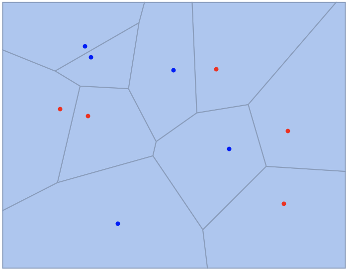
Here is how to create a Voronoi diagram with different colored points that represent offensive and defensive players.
pt = RandomReal[{0, 10}, {10, 2}];(*creates a 10 by 2 array of points between 0 and 10*)
Show[
 VoronoiMesh[pt],
 Graphics[{PointSize@Medium, Red, Point[pt[[1 ;; 5]]], Blue,
   Point[pt[[6 ;; 10]]]}]
 ](*creates the diagram showing the points and the cells*)
1st Trial
Using the NearestNeighborGraph to connect the offensive points
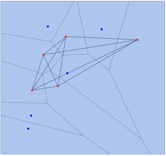
This was one of my methods used to find a way that best optimizes the offense. The idea for this method was to use the NearestNeighborGraph function to create a polygon by connecting all the offensive(red) points. This will allow for us to calculate the area of the polygon which was created by all the offensive points.
ptt = RandomReal[{0, 10}, {10, 2}];(*creates a 10 by 2 array of points between 0 and 10*)
ntt = NearestNeighborGraph[ptt[[1 ;; 5]], 4];(*finds the 4 nearest neighbors of the offensive(red)points*)
Show[
 Show[
  VoronoiMesh[ptt], ntt
  ],
 Graphics[{
   PointSize@Medium, Red, Point[ptt[[1 ;; 5]]],
   Blue, Point[
    ptt[[6 ;; 10]]]}](*creates the colored points- red for offense, blue for \
defense*)
 ]
The result:
Now we could find the area of the polygon created from the connected offensive(red) points.
ptt //
  Polygon@# & //
 RegionMeasure@# &
This should return 10.145, the area of the polygon from the previous code.
We can infer that the area is significant because a greater area created from these offensive points allow for more space for the offensive players to interact. A greater area created from the offensive players also infers that less space is taken up on the court by the defensive(blue) points and more space is taken up by the offensive points. Later, I found out this method was not as efficient as other methods and had some errors such as the points not being in realistic positions like it would be on a real basketball court.
So what next...
Once I realized that the previous method wasn't as good as I hoped it would have been, I quickly needed to find another way. So I went to my mentor. My mentor gave me a lot of information and ways I could further improve the situation.
Connected Components Function (2nd method)
This function allows the user to input their points into the function, creating a Voronoi diagram of the offensive and defensive players separated by the red and blue color. The user-inputted points can allow the user to choose which players are on offense and defense, allowing for more interaction between the user and the code. It will also provide the area of the respective colors cells, giving the user the information needed to infer a conclusion from the function.
The FUNCTION
connectedComp[points_] :=
 Block[{off, def, oprims, oconnect, dconnect, a, b},
  VoronoiMesh[points](*Voronoi Mesh creates Voronoi cells out of the \
specified points*)//
     MeshPrimitives[#, 2] &(*this line generates the polygon coordinates created by \
each cell*)//
    #[[
       Ordering[(*orders the list by giving the position of the order*)
        Position[(*finds the position where the RegionMember \
returns true*)
          Outer[(*This will return a list of True or False depending \
on if the points in the Voronoi cells are located inside the region \
of the polygons created from MeshPrimitives[VoronoiMesh[points] ,2]*)
           RegionMember,
           MeshPrimitives[
            VoronoiMesh[points] , 2],
           points,
           1]
          , True][[All, 2]]
        ]
       ]] & //
   (oprims = #) &;

  off =
   Flatten[
    oprims[[1 ;; Length[points]/ 2]] //(*creates the offensive points(5 points)*)
       SimpleGraph@RelationGraph[
          Not@*RegionDisjoint,(*This provides a graph of the edges
and vertices of the points when the polygons are not disjoint*)
    #,
          VertexLabels -> None] & //
      ConnectedComponents@# & //(*This line connects the components \
of the relation graph*)
     (oconnect = #) &];(*returns the first five(offensive)points*)

  def =
   Flatten[
    oprims[[Length[points]/2 + 1 ;; -1]] //(*creates the defensive points(5 points)*)
       SimpleGraph@RelationGraph[
          Not@*RegionDisjoint,(*This provides a graph of the edges
and vertices of the points when the polygons are not disjoint*)
    #,
          VertexLabels -> None] & //
      ConnectedComponents@# & //(*This line connects the components \
of the relation graph*)
     (dconnect = #) &];(*returns the last five(defensive)points*)

  a = MaximalBy[
     oconnect,
     Total[Area /@ #] &
     ] // First(*connected area of offensive team*);
  b = MaximalBy[
     dconnect,
     Total[Area /@ #] &
     ] // First(*connected area of defensive team*);

  red = RGBColor["#E86850"];
  blue = RGBColor["#587498"];

  Show[Graphics[
    {EdgeForm[Black],
     Lighter@blue, Complement[def, b],
     Lighter@red, Complement[off, a],
     blue, b,
     red, a,
     Black, PointSize@Medium, Point[points]},
    PlotLabel ->
     Grid[{{"Total Area of Offense: " <>
         ToString[
          Total[RegionMeasure /@ off]/(Total[RegionMeasure /@ off] +
             Total[RegionMeasure /@ def])],
        "Total Area of Defense: " <>
         ToString[
          Total[RegionMeasure /@ def]/(Total[RegionMeasure /@ off] +
             Total[RegionMeasure /@
               def])]}, {"Area of Connected Offensive Cells: " <>
         ToString[
          Total[RegionMeasure /@ a]/Total[RegionMeasure /@ off]],
        "Area of Connected Defensive Cells: " <>
         ToString[
          Total[RegionMeasure /@ b]/Total[RegionMeasure /@ def]]}},
      Frame -> All, FrameStyle -> {Thick, Directive[Black]}]]]](*This graphic will show the Voronoi diagram and create a frame with the areas of the respective regions inside*)
Here is a random example of what the function returns:
connectedComp[RandomReal[{0,10},{10,2}]]
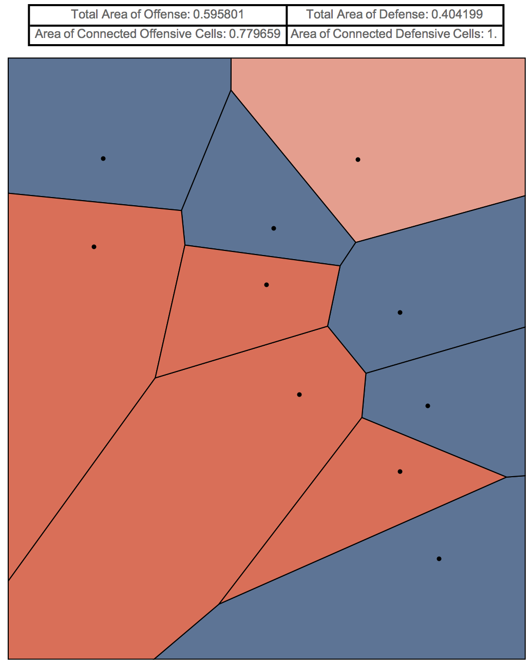
The user could also input their own points:
connectedComp[{{0.4, 1}, {1.4, 1.4}, {4.6, 2.5}, {8.5, 2.1}, {9.4, 8.6}, {0.5, 0.6}, {3.4, 0.9}, {6.2, 1.2}, {8.2, 0.4}, {9.7, 0.2}}]
Which will return:
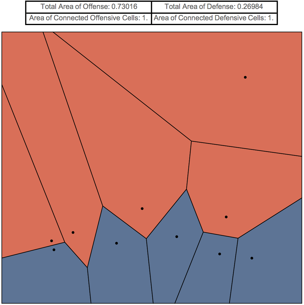
This is an example of an efficient offense because of the large offensive area.
This is an example of an inefficient offense because of the large connecting area of the defensive cells.
connectedComp[{{0.5, 0.2}, {3.4, 0.2}, {6.2, 0.5}, {8.2, 1.4}, {9.7, 0.2}, {0.4, 9.4}, {1.4, 1.4}, {5, 2.5}, {8.7, 2.1}, {9.4, 0.2}}]
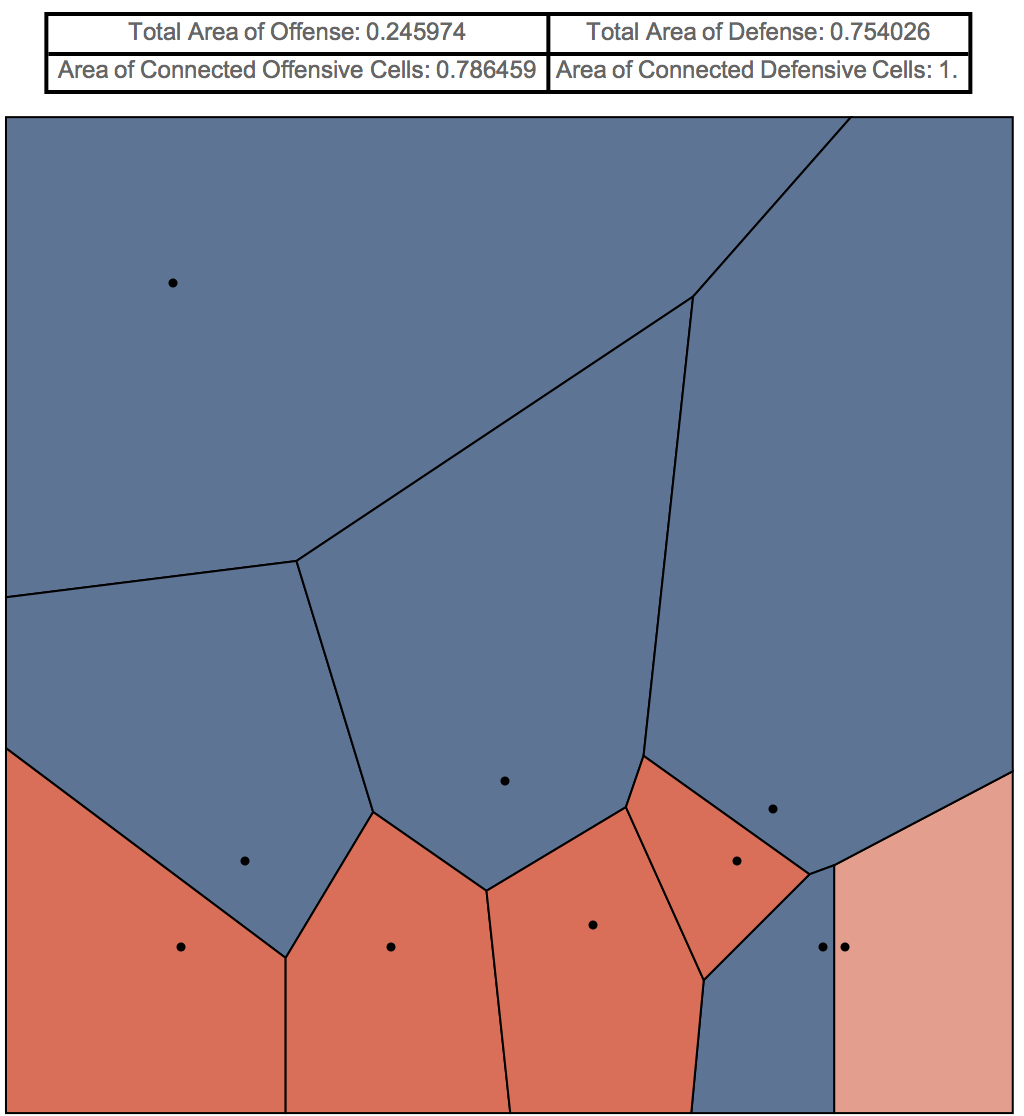
Conclusion
This function provides a very detailed diagram of the interaction between the offensive and defensive players. The red-colored cells represent the offensive players, while the blue-colored cells represent the defensive players. The lighter-colored red cells represent the offensive cells that are not connected to the rest of the the offensive cells, while the lighter-colored blue cells represent the defensive cells that are not connected to the rest of the defensive cells. The diagram also gives information about the area, in percentage, of the offensive and defensive cells. It will give you a decimal number that is determined from the area of the total offensive or defensive cells divided by the total of both the offensive and defensive cells, which represents how much space either the offense or defense covers on the court. It also provides us with data on the area of the connecting cells of offensive or defensive players. The graphic will show us a decimal number which represents the greatest connecting area for each side, calculated from maximum connected area of one side divided by the total area of that side.
All of this information is significant because the greater total area of the offense allows for the offense to cover up more space on the court than the defense, giving them a better opportunity to score or advance the ball. However, a greater total area of the defense gives the offense a smaller opportunity to get a good shot and effectively run their plays. The area of connecting offensive cells shows how much space the offense could utilize without being interfered by the defense, so a greater area of connecting offensive cells would be better for optimizing the offense.
Future Work
Some of the ideas in the project have room for improvement. For example, I could make it to be more user-friendly. Instead of making the user enter the points for both the offense and defense, I could use the Locator function to allow the user to drag the defense to wherever the user wants and then place the offensive points at the most optimal places based on the defense the user chose. I also could have used a more efficient code by creating a code that will use less space and make the runtime faster.
 Attachments:


