Greetings,

The focus of this post is going to be how we can use the Wolfram language and Mathematica to better visualize the shapes present in a given Moire pattern. First, we will briefly review what Moire patterns are, and how to build one in Mathematica. Then, we will look at the different functions that allow us to see the shapes inside Moire patterns better. Lastly, we will use these functions to create interesting Manipulate and Cloud objects.

Introduction to Moire patterns

The basic definition of a Moire pattern is: A pattern that can be observed when a ruled pattern with is overlaid with another rotated/displaced version of the same (or similar) pattern. They are not only mesmerizing to watch, but have real life uses as well. For example in Physics, where a pattern is projected on a surface. The surface is then modified, and so the projected pattern changes. Both, the new and the original pattern are overlaid. Scientists can look at the resulting Moire pattern to determine the change in the surface. Here is a an example of a Moire Pattern:

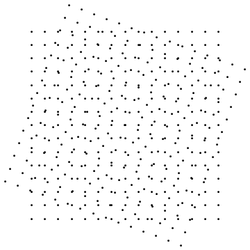
This example, built with Mathematica, shows a set of equidistant points, overlaid by the same set, rotated 70 Degrees. The code to do so was:

pts = Table[Point[{x, y}], {x, -7, 7}, {y, -7, 7}];
Graphics[{pts, Rotate[pts, 70 Degree]}]

First, we generate the set of points (pts), and then we rotate it using the function Rotate.

In Mathematica you can not only generate moire patterns based on sets of points, but you can do so with other shapes as well. Let's take lines for example:

lines = Table[Line[{{x, 0}, {x, 1}}], {x, 0, 1, 0.05}];
Graphics@Table[Rotate[lines, r], {r, \[Pi]/5, \[Pi], \[Pi]/5}]

The resulting Moire Pattern would be:

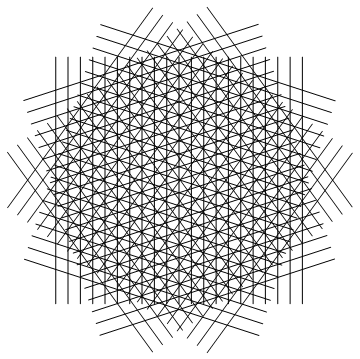
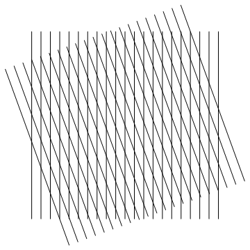
In this particular example, we generated a table of sets of lines, instead of just using 2. There is no special reason to it, it's just so it looks better. You can do it with just two sets aswell:

lines = Table[Line[{{x, 0}, {x, 1}}], {x, 0, 1, 0.05}];
Graphics[{lines, Rotate[lines, 20 Degree]}]

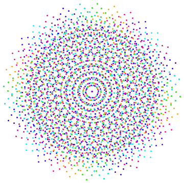
You can also play around with Manipulate and Moire patterns. A cool example would be:

points = Table[Point[{x, y}], {x, -10, 10}, {y, -10, 10}];
Manipulate[Graphics[Table[Rotate[Style[points, Hue[a]], a], {a, a, 4 a, \[Pi]/16}]], {a, 0, \[Pi]/4}]

Beware: This Manipulate may require quite a bit of computing

The result should look something like this:

Making shapes in Moire patterns more visible

Mathematica has an array of different functions used to analyze images and graphics. I explored a few of them and found out that the best functions to visualize the shapes inside Moire patterns were SkeletonTransform and VoronoiMesh. Also, I looked at Histogram3D to see how the density of the points in a Moire pattern changed over time.

Let's start with the function Skeleton. Before using it, we must convert the graph into an image, because Skeleton only takes images as Arguments. To do so, we just use Rasterize

graph=With[{points = Table[Point[{x, y}], {x, -15, 15}, {y, -15, 15}]}, Graphics[{points, Rotate[points, 70]}]];
img=Rasterize[graph]

Note: Instead of defining pts to do the graph, we can use the function With, as used in the last code

Now that we have an image, we can use SkeletonTransform to get the shapes. We will also crop the image so it's easier to see the shapes.

SkeletonTransform[ImageCrop[img, Round[ImageDimensions[img]/2]]] // ImageAdjust

The output should look like this:

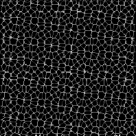
SkeletonTransform does a good enough job representing the shapes, but there is another function that represents them better/clearer. It is called VoronoiMesh and it generates a Mesh, consisting of cells around the points it is given. To use this function, we need to use another Method of rotating the points. So, instead of using Rotate as we did before, we will use RotationTransform to get the coordinates of the rotated points. We will crop the image as we did with SkeletonTransform, just so the shapes are clearer.

points = Table[Point[{x, y}], {x, -10, 10}, {y, -10, 10}];
r = RotationTransform[\[Pi]/4];
rotatedpoints = points /. Point -> r;
finalpoints = rotatedpoints /. {x_, y_} -> Point[{x, y}];
setofpoints = Join[points, finalpoints];
densitypoints = setofpoints /. Point[{x_, y_}] -> {x, y};
flat = Flatten[densitypoints, 1];
i = VoronoiMesh[flat, PlotTheme -> "Lines"];
image = Rasterize[i];
ImageCrop[image, Round[ImageDimensions[image]/2]] // ImageAdjust

The output should look like this:

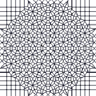
Note: Try different angles to get different shapes. (The angle in this code is determined by the argument of RotationTransform)

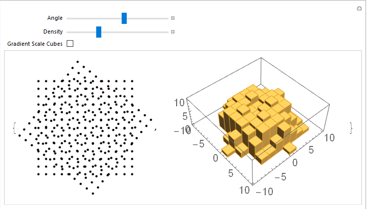
I talked about how we could use Histogram3D to see how the density of the points changed with each angle. There are two ways to approach this. You can make a function and manually change the angle to get each Histogram3D for each given angle, or you could do a Manipulate to slide and see how it changes. I took the second approach and added a graph of the Moire pattern in itself to better visualize the change.

Here is the code for the Manipulate:

Manipulate[
 Module[
  {MoireHistogram, graph},
  MoireHistogram[a_] := 
   Module[{points, r, rotatedpoints, finalpoints, setofpoints, 
     densitypoints, flat2},
    points = Table[Point[{x, y}], {x, -d, d}, {y, -d, d}];
    r := RotationTransform[a];
    rotatedpoints := points /. Point -> r;
    finalpoints := rotatedpoints /. {x_, y_} -> Point[{x, y}];
    setofpoints := Join[points, finalpoints];
    densitypoints := setofpoints /. Point[{x_, y_}] -> {x, y};
    flat2 := Flatten[densitypoints, 1];
    If[gd,
     Histogram3D[flat2, Automatic, 
      ChartElementFunction -> "GradientScaleCube"],
     Histogram3D[flat2]]
    ];
  graph[a_] := 
   With[{points = Table[Point[{x, y}], {x, -d, d}, {y, -d, d}]}, 
    Graphics[{points, Rotate[points, a]}]];
  {Magnify[graph[a], 1.5], Magnify[MoireHistogram[a], 2]}],
 {{a, \[Pi]/4, "Angle"}, 0, \[Pi]/2},
 {{d, 4, "Density"}, 2, 15, 1},
 {{gd, False, "Gradient Scale Cubes"}, {True, False}}
 ]

And here is a snapshot of the end product:

Interesting Manipulate and Cloud objects

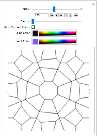
We have already seen some Manipulate objects, but there is more to it. For example, with Mathematica, you can create a Manipulate that lets you change the angle, point density and color of a VoroniMesh from a moire pattern, all in the same Manipulate:

Manipulate[
{Module[
   {points, r, rotatedpoints, finalpoints, setofpoints, densitypoints,
     flat},
   points = Table[Point[{x, y}], {x, -d, d}, {y, -d, d}];
   r = RotationTransform[a];
   rotatedpoints = points /. Point -> r;
   finalpoints = rotatedpoints /. {x_, y_} -> Point[{x, y}];
   setofpoints = Join[points, finalpoints];
   densitypoints = setofpoints /. Point[{x_, y_}] -> {x, y};
   flat = Flatten[densitypoints, 1];
   If[showpoints,
    i = Graphics[{co, 
       MeshPrimitives[VoronoiMesh[flat, PlotTheme -> "Lines"], 1], 
       co2, Point[flat]}],
    i = Graphics[{co, 
       MeshPrimitives[VoronoiMesh[flat, PlotTheme -> "Lines"], 1]}]];
   image = ImageResize[Rasterize[i, ImageResolution -> 100], "Large"];
   Magnify[ImageCrop[image, Round[ImageDimensions[image]/2]], 3]
   ]},
 {{a, \[Pi]/4, "Angle"}, 0, 1.569},
 {{d, 4, "Density"}, 2, 17, 1},
 {{showpoints, False, "Show Voronoi Points"}, {True, False}},
 {{co, Black, "Line Color"}, Black},
 {{co2, Orange, "Point Color"}, Orange}
 ]

And the corresponding snapshot:

Moving on to the Cloud objects, we can create a Microsite that receives an angle and a point density, to return a Moire pattern and its Voronoi Mesh. To do so we need to first define a function, then a FormFucntion and lastly CloudDeploy that FormFunction.

func1[a_, d_] := 
 Module[{MoireVoD, graphD}, 
  MoireVoD[a, d] := 
   Module[{points, r, rotatedpoints, finalpoints, setofpoints, 
     densitypoints, flat},
    points = Table[Point[{x, y}], {x, -d, d}, {y, -d, d}];
    r = RotationTransform[a];
    rotatedpoints = points /. Point -> r;
    finalpoints = rotatedpoints /. {x_, y_} -> Point[{x, y}];
    setofpoints = Join[points, finalpoints];
    densitypoints = setofpoints /. Point[{x_, y_}] -> {x, y};
    flat = Flatten[densitypoints, 1];
    i = VoronoiMesh[flat, PlotTheme -> "Lines"];
    image = Rasterize[i];
    ImageCrop[image, Round[ImageDimensions[image]/2]] // ImageAdjust
    ];
  graphD[a, d] := 
   With[{points = Table[Point[{x, y}], {x, -d, d}, {y, -d, d}]}, 
    Graphics[{points, Rotate[points, a]}]];
  {graphD[a, d], MoireVoD[a, d]}]
form1 = FormFunction[{"a" -> "Real", "d" -> "Integer"}, 
  func1[#a, #d] &, 
  AppearanceRules -> <|"Title" -> "Moire and Voronoi", 
    "Description" -> 
     "Enter an Angle (a) between 0 and 1.569 (Radians) and a point \
density (d) between 4 and 17 to receive a Moire Pattern with its' \
corresponding Voronoi Mesh"|>]
CloudDeploy[form1, "Moire and Voronoi", Permissions -> "Public"]

You can click here to go to the Microsite.

Conclusions

We have seen how Mathematica has different ways to display the same data, in this case, how it can display the information given by a Morie pattern. I am sure that I missed a couple of functions, so, if you have any suggestions for which other functions might represent Moire patterns better, feel free to discuss them in the reply section. Also, if you think anything in this post could have been done better, do not hesitate and reply. All feedback is greatly appreciated.