NOTE: all Wolfram Language code and data are available in the attached notebook at the end of the post.
Novel method for volatility objects building is being discussed in the attached note. Machine learning techniques are being applied to financial derivatives volatility building and the method of predictions fits sample data well. The resulting objects are reasonable, they build fast and produce logically correct estimates within given domains. As such, data science route offers interesting alternative to traditional modelling assumptions.
Introduction
Volatility plays critical role in the modelling and valuation of financial derivatives, and therefore it is not surprising to see continuous attention and focus of many quants and researchers alike on this subject, pattern decomposition and process modelling. Knowing the 'right' volatility and being able to estimate its path in the future is therefore seen as critical ingredient of consistent derivatives pricing.
Financial volatilities are either given (quoted by the broker-dealers) or implied (derived from option prices). By its nature, financial products volatilities are generally 'forward-looking' rather than being historical / realised volatilities. This phenomenon stems from the principles of risk-neutral pricing. When the volatility is quoted, its origin is in many instances derived from volatility models. These can be simple (such as B/S) or more complex. Local volatility SABR and the 'mixture' models such as SVLV are currently the most used volatility models in the market. To operate properly, all these models require extensive calibration to the market data.
We propose alternative method for volatility object building that utilises data science approach. Using Mathematica's routines for machine learning, we use predictor functionality to build volatility oaths based on 'learning' from quoted data. We will look at three volatility objects - FX, Equity and Interest rate swaptions to show Mathematica's capabilities in the construction and management of volatility objects by 'learning' from given examples. The method is generally fast and can be fully automated. This improves its usability and future application in quantitative finance.
FX Volatility
FX volatility is quoted in the market either in 1D or 2D directions. The former is generally a vector of at-the-money (ATM) volatilities for different option maturities, whilst the latter is a 2D surface that in addition to maturity dimension introduces option strikes. These are generally shown on horizontal axis with quoted expression as FX delta. 50 delta is equal to ATM, 10 and 25 delta represent out-of--the money (OTM) calls whilst 75 and 90 reflect puts. The non-negativity of FX market leads to a log-normal assumptions about the FX data distribution, and therefore the nature of quoted volatility is log-normal (or also known as relative volatility).
We use the recent FX volatility data for JPY/BRL currency cross. Option maturity range from 1 day to 10 years and the FX smile is defined for both calls and puts on the above strike scale.
fxmat = {1/360, 7/360, 14/360, 21/360, 30/360, 60/360, 90/360,
   120/360, 150/360, 180/360, 1, 1.5, 2, 3, 4, 5, 7, 10};
fxdelta = {10, 25, 50, 75, 90};
xtbl = Table[{i, j}, {i, fxmat}, {j, fxdelta}] // Transpose;

fxvols0 = {{28.9347360822946, 23.266, 18.69473828125, 17.336,
    17.082}, {22.817, 18.889, 18.7004305555556, 14.768,
    14.435}, {22.462, 18.476, 18.6928159722222, 14.352,
    14.026}, {22.741, 18.775, 18.6928532986111, 14.673,
    14.356}, {23.885, 20.609, 18.6928532986111, 17.419,
    17.814}, {23.41, 20.449, 18.6928159722222, 17.174,
    17.161}, {23.811, 20.843, 18.7004305555556, 17.395,
    17.229}, {24.998, 21.005, 18.6759444444444, 17.188,
    17.089}, {23.849, 20.471, 18.7022222222222, 16.766,
    16.488}, {23.107, 20.095, 18.6926666666667, 16.466,
    16.117}, {23.099, 19.807, 18.7308888888889, 15.833,
    15.346}, {22.2539294889054, 20.404, 18.578, 16.29,
    15.8708687695123}, {22.7761138678155, 20.642, 18.8, 16.449,
    16.1821988373345}, {22.0841109536103, 20.326, 18.7, 16.059,
    15.4239471417806}, {22.6021123295428, 20.563, 18.6926666666667,
    16.158, 15.6147034126386}, {21.4177604234308, 20.017,
    18.7308888888889, 15.563, 14.4858894630447}, {22.4813659703195,
    20.508, 18.7078518518519, 15.849,
    15.023193562278}, {23.0150689352065, 20.75, 18.7104691358025,
    16.003, 15.3165637372759}};
fxvols = fxvols0 // Transpose;
The FX volatility surface looks as follows:
TableForm[fxvols // Transpose, TableHeadings -> {fxmat, fxdelta}]
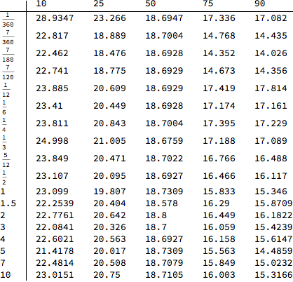
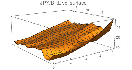
We can visualise it as follows:
ListPlot3D[fxvols, PlotLabel -> Style["JPY/BRL vol surface", 14]]
Training predictor on the FX volatility data
We use the quoted volatility data as a 'training set' to discover the pattern in the data for predictor purposes. Predict function is our main tool for this task and we build two objects:
- Vol object with Gaussian process method
- Vol object with Random forest method
We first build the training set object and format it in required direction
fxvoldata0 =
  Table[{fxmat[[i]], fxdelta[[j]]} -> fxvols[[j, i]], {j, 1,
    Length[fxdelta]}, {i, 1, Length[fxmat]}];
fxvoldata1 = Flatten[fxvoldata0, 1];
Using the data object, we now train two predictors:
fxvmodelGP =
 Predict[fxvoldata1, PerformanceGoal -> "Quality",
  Method -> "GaussianProcess"]
fxvmodelRF =
 Predict[fxvoldata1, PerformanceGoal -> "Quality",
  Method -> "RandomForest"]

and examine the information about each predictor function
{PredictorInformation[fxvmodelGP],
  PredictorInformation[fxvmodelRF]} // Row

We can now test the predictors on same sample data:
{fxvmodelGP[{7, 10}], fxvmodelRF[{7, 10}], fxvmodelGP[{1/2, 50}],
 fxvmodelRF[{1/2, 50}]}
{22.2577, 22.2484, 18.6702, 18.6932}
We observe decent fit to the original data. Using the model, we can now build the entire volatility object, filling the gaps in the quoted spectrum:
fxmodres =
  Table[{i, j, fxvmodelGP[{i, j}]}, {i, 0.5, 10, 0.25}, {j, 5, 95, 5}];
fxmoevals = Flatten[fxmodres, 1];
ListPlot3D[%,
 PlotLabel ->
  Style["Predicted FX Vol Surface: Gaussian Process approach", Blue,
   Italic, 15], AxesLabel -> {"Tenor", "Delta"},
 ColorFunction -> "Rainbow", ImageSize -> 400]
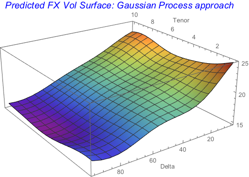
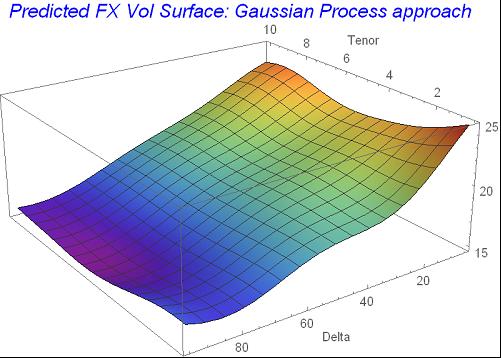
Gaussian process model builds smooth and well-behaved volatility surface in both dimensions. The model nicely smooches the edges observed in the original data
fxmodres2 =
  Table[{i, j, fxvmodelRF[{i, j}]}, {i, 0.5, 10, 0.25}, {j, 5, 95,
    10}];
Flatten[fxmodres2, 1];
ListPlot3D[%, ColorFunction -> "TemperatureMap",
 PlotLabel ->
  Style["Predicted FX Vol Surface: Random Forest approach", Blue,
   Italic, 15], AxesLabel -> {"Tenor", "Delta"},
 ColorFunction -> "TemperatureMap", ImageSize -> 400]
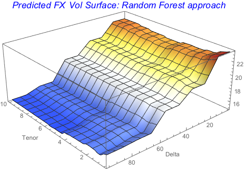
The nature of the Random forest model means that the modelled surface looks step-wise. If the smoothness is preferable for the vol object construction, then Gaussian process is a better choice.
Equity volatility
We now look at the Equity volatility data and will build vol objects in a similar way to the FX case above. Equity volatility data exist in the 2D surface format : (i) in option maturity dimension and (ii) option strike dimension. In this way they closely resemble the FX volatilities. By nature, the equity volatilities are also log-normal since equity prices are always positive.
Equity options maturity typically range from 1 month up to 5 years, whereas option strikes - expressed in terms of 'moneyness' - range between 40 and 200%.
We take the recent Nikkei 225 equity volatility data defined on the grid mentioned above:
eqdates = {1/12, 2/12, 3/12, 6/12, 1, 3/2, 2, 3, 4, 5};
eqmoney = {0.4, 0.6, 0.8, 0.9, 0.95, 0.975, 1, 1.025, 1.05, 1.1, 1.2,
   1.3, 1.5, 1.75, 2};
eqv = {{54.743, 42.171, 33.275, 24.208, 20.015, 17.999, 16.541,
    15.679, 15.173, 15.752, 18.185, 20.298, 24.619, 27.651,
    29.413}, {46.068, 39.862, 29.681, 22.664, 19.624, 18.228, 17.138,
    16.358, 15.777, 15.358, 16.869, 18.244, 21.776, 24.987,
    27.007}, {42.368, 38.084, 27.929, 22.151, 19.673, 18.547, 17.639,
    16.995, 16.55, 16.053, 16.726, 17.704, 20.029, 23.105,
    25.135}, {42.136, 34.798, 25.302, 21.623, 19.971, 19.281, 18.721,
    18.289, 17.966, 17.57, 17.655, 18.439, 19.792, 21.623,
    23.704}, {38.829, 30.246, 23.945, 21.428, 20.393, 19.97, 19.614,
    19.322, 19.087, 18.762, 18.574, 18.876, 19.975, 21.059,
    22.035}, {35.555, 28.012, 23.123, 21.135, 20.363, 20.046, 19.775,
    19.547, 19.358, 19.079, 18.844, 18.951, 19.739, 20.737,
    21.493}, {33.111, 26.718, 22.555, 20.905, 20.28, 20.022, 19.799,
    19.608, 19.446, 19.198, 18.952, 18.968, 19.518, 20.418,
    21.127}, {30.028, 25.228, 21.861, 20.629, 20.171, 19.981, 19.813,
    19.667, 19.54, 19.339, 19.108, 19.058, 19.347, 20.034,
    20.687}, {28.217, 24.273, 21.397, 20.413, 20.049, 19.896, 19.761,
    19.641, 19.536, 19.366, 19.156, 19.084, 19.245, 19.765,
    20.341}, {26.918, 23.453, 20.936, 20.115, 19.812, 19.683, 19.568,
    19.466, 19.376, 19.227, 19.033, 18.952, 19.04, 19.439, 19.936}};
eqvols = eqv // Transpose;
TableForm[eqv, TableHeadings -> {eqdates, eqmoney}]
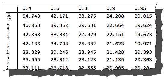
This is the equity volatility surface quoited in the market
eqtab = Table[{eqdates[[i]], eqmoney[[j]], eqv[[i, j]]}, {i, 1,
    Length[eqdates]}, {j, 1, Length[eqmoney]}];
Flatten[eqtab, 1];
ListPlot3D[%, PlotLabel -> Style["Nikkei 225 vol surface", 14]]
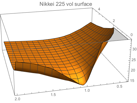
The skew above is a typical feature of the equity markets.
Training predictor on the Nikkei volatility data
We first configure the vol data object for the modelling purposes
eqs = Table[{eqdates[[i]], eqmoney[[j]]} -> eqv[[i, j]], {i, 1,
    Length[eqdates]}, {j, 1, Length[eqmoney]}];
eqdataset = Flatten[eqs, 1];
and then train two predictors:

Obtain information about each method:
{PredictorInformation[eqvolmodelGP], PredictorInformation[eqvolmodelNN]}
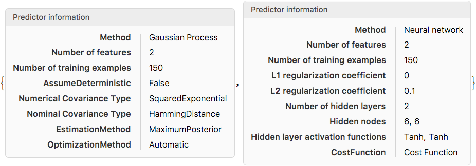
We test each predictor on a sample data
{eqvolmodelGP[{1, 0.6}], eqvolmodelNN[{1, 0.6}], eqvolmodelGP[{3, 2}], eqvolmodelNN[{3, 2}]}
{29.8471, 31.0239, 20.6998, 20.9776}
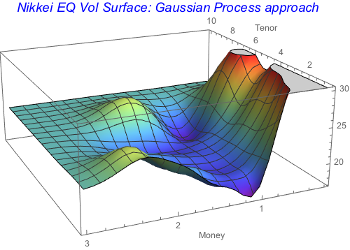
We can see a decent fit to the original data. We now generate the full volatility surface by extending the boundaries outside the original domain:
eqmodres =
  Table[{i, j, eqvolmodelGP[{i, j}]}, {i, 0.5, 10, 0.25}, {j, 0.2, 3,
    0.1}];
eqmodres = Flatten[eqmodres, 1];
ListPlot3D[%,
 PlotLabel ->
  Style["Nikkei EQ Vol Surface: Gaussian Process approach", Blue,
   Italic, 15], AxesLabel -> {"Tenor", "Money"},
 ColorFunction -> "Rainbow", ImageSize -> 400]
eqmodres =
  Table[{i, j, eqvolmodelNN[{i, j}]}, {i, 0.5, 10, 0.25}, {j, 0.2, 3,
    0.1}];
eqmodres = Flatten[eqmodres, 1];
ListPlot3D[%,
 PlotLabel ->
  Style["Nikkei EQ Vol Surface: Neural network approach", Blue,
   Italic, 15], AxesLabel -> {"Tenor", "Money"},
 ColorFunction -> "TemperatureMap", ImageSize -> 400]
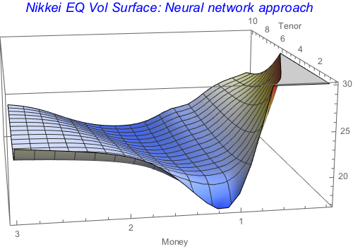
Both predictors produce smooth volatility objects, with Neural network being closer to the underlying data.
Swaption cube
Our third example is based on more complex case - 3D swaption cube. Interest rate swaptions are defined on 3D scale - (i) option maturity, (ii) underlying swap maturity and (iii) strike. This makes the case more complicated. Option maturities range from 1month to 30 years, swap maturities are typically between 1year and 30 years and strikes are usually in the range of -200 to 200 where the number represents the basis point offset from ATM swap rate.
Since in many currencies the rates are now negative, the market has moved from quoting the log-normal volatilities to the normal ones. These are also known as 'absolute' volatilities and are usually expressed on rates convention basis.
We take the recent EUR swaption volatility data and create training set for the Mathematica's predictor:
optmat = {1/2, 3/4, 1, 2, 3, 4, 5, 6, 7, 8, 9, 10, 12, 15, 20, 25, 30};
swmat = {1, 2, 3, 4, 5, 6, 7, 8, 9, 10, 12, 15, 20, 25, 30};
swox = {-200, -150, -100, -75, -50, -25, 0, 25, 50, 75, 100, 150,  200};

Fully-defined cubes, such as the EUR one are generally large:
Map[Length, swv] // Total
3315
Training the predictor on the EUR swaption volatility data
We first build the vol object from the data
swvres1 =
  Table[{optmat[[i]], swmat[[k]], swox[[j]]} -> swv[[i, j]], {k, 1,
    Length[swmat]}, {j, 1, Length[swox]}, {i, 1, Length[optmat]}];
swvres2 = Flatten[swvres1, 2];
and create three predictors:

    swvolmodNN =
     Predict[swvres2, Method -> "NeuralNetwork",
      PerformanceGoal -> "Quality"]

    swvolmodRF =
     Predict[swvres2, Method -> "RandomForest",
      PerformanceGoal -> "Quality"]

Whilst the Neural network and Random forest are generally fast to build, the Gaussian process is slower
{Predict[swvres2, Method -> "GaussianProcess",
   PerformanceGoal -> "Quality"] // Timing,
 Predict[swvres2, Method -> "NeuralNetwork",
   PerformanceGoal -> "Quality"] // Timing,
 Predict[swvres2, Method -> "RandomForest",
   PerformanceGoal -> "Quality"] // Timing}

We test the predictors on the sample data
{swvolmodGP[{10, 1, 0}], swvolmodNN[{10, 1, 0}],
 swvolmodRF[{10, 1, 0}]}
{0.698667, 0.698477, 0.69649}
We again observe decent fit to the original data.
Using the three vol models, we predict the volatility data and fill the cubes:
volmodGP =
  Table[swvolmodGP[{i, j, k}], {i, 1, 5, 0.5}, {j, 1, 10,
    1}, {k, -100, 100, 50}];

volmodNN =
  Table[swvolmodNN[{i, j, k}], {i, 1, 10, 0.25}, {j, 1, 10,
    1}, {k, -200, 200, 25}];

volmodRF =
  Table[swvolmodRF[{i, j, k}], {i, 1, 10, 0.25}, {j, 1, 10,
    1}, {k, -200, 200, 25}];

{ListPlot3D[Table[volmodNN[[i]], {i, Length[volmodNN]}],
  ColorFunction -> "Rainbow",
  PlotLabel -> Style["EUR Swaption cube: NN approach", 12],
  AxesLabel -> {"Opt Tenor", "Swap Tenor"}, ImageSize -> 250],
 ListPlot3D[Table[volmodGP[[i]], {i, Length[volmodGP]}],
  ColorFunction -> "TemperatureMap",
  PlotLabel -> Style["EUR Swaption cube: GP approach", 12],
  AxesLabel -> {"Opt Tenor", "Swap Tenor"}, ImageSize -> 250],
 ListPlot3D[Table[volmodRF[[i]], {i, Length[volmodRF]}],
  ColorFunction -> "NeonColors",
  PlotLabel -> Style["EUR Swaption cube: RF approach", 12],
  AxesLabel -> {"Opt Tenor", "Swap Tenor"}, ImageSize -> 250]}

All three predictors correctly show the flattening of the surfaces for higher strikes. Neutral network produces the smoothest surface, and additionally is the fastest to build the object. As such, it may be well suitable for live market data and active volatility management.
Conclusion
The objective of this note was to show that machine learning method offered viable alternative to traditional volatility models using single or multi-factor processes.. Data science approach is attractive as it actively 'learns' from available data samples and adjusts its parameters when either market conditions or direction change. Built-in Mathematica's Predict function provides excellent routines for volatility data fitting and three tested methods provide reasonable prediction for the modelled data. More importantly, higher dimensions, such as cubes, pose no problem for object rendering. This remains robust and fast.