Making a Christmas Animation with the Wolfram Language

This notebook describes how to build an animation of a decorated pine tree that moves its branches synchronized to the voices of the music of the 16th century German O Tannenbaum song (the English version is O Christmas Tree). One dedicated branch of the tree will act as the conductor and a candle will be the baton. The keep the animation interesting through all versus we will also add some snowfall and some ecstatic tree movements in the second half of the song. To see the final design watch this YouTube video:

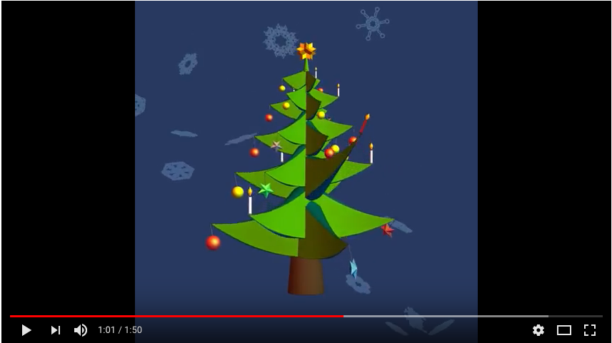
I will implement the animation through the following steps:

1) Build a pine tree with curved branches where the branches can be moved smoothly up and down and left and right.

2) Add ornaments (colored balls, five-pointed stars) and candles of different color to the branches. Allow the ornaments to be moved with respect to the branch tips.

3) Convert the 4 voices of the music to a 2D movement based on the frequencies of the sound. Model the conductor movements in sync with the music.

4) Model the movements of the ornaments as forced spherical pendula. Account for friction of the ornaments using the Rayleigh dissipation function.

5) Add some snowfall for having a white Christmas.

6) Build the animation with the branches using according to the music.

Special thanks to my coworker Andrew Steinacher for selecting the music and analyzing the music to get the data for the tree movements (the below section From Music to Movements). And thanks to Amy Young for turning the animation frames and the music into one video clip.

Making a Pine Tree

Tree Parameters

The tree dimensions, the overall shape of the tree and counts of branches. The variable names make their meaning obvious.

(* radial branch count *)
radialBranchCount = 3;
(* vertical branch count *)
verticalBranchCount = 5;
(* tree height *)
treeHeight = 12;
(* tree width *)
treeWidth = 6;

(* plot points for the B-spline surfaces forming the branches *)
{?, ?} = {6, 8}; 

Colors of stem and branches.

stemColor = Directive[Darker[Brown], Lighting -> "Neutral", Specularity[Brown, 20]];
branchTopColor = RGBColor[0., 0.6, 0.6];
branchBottomColor = RGBColor[0., 0.4, 0.4];
branchSideColor = RGBColor[0.4, 0.8, 0.];

Grow a Movable Tree Branch

Each branch has a rectangle cross section with changing dimension (as a function of the distance from the stem). The tip of the branch should be pointing slightly upwards to have the iconic shape of a Christmas tree. At its widest size, the branch is made to fit smoothly to a cone (the stem). The variable $\tau$ determines the up-down and variable $\sigma$ the left-right position of the tip of the branch. I build a branch from four B-spline surfaces (top, bottom, left, right) to have a smooth appearance with only a small number of points defining the surface.

branchTopBottom[
  tp_, {hb_, ht_}, {?1_, ?2_}, {rb_, rt_}, 
  R_, {?_, ?_}] := 
 Module[{A = -0.6, ? = 1/2, ?m, Pm, dirR, 
   dir?, r, P1, P, \[ScriptN], \[ScriptP], x, 
   y, ?, ?, ?, \[ScriptH]s, \[ScriptH]},
  ?m = Mean[{?1, ?2}]; 
  Pm = R {Cos[?m], Sin[?m]}; 
  dirR = 1. {Cos[?m], Sin[?m]};
  dir? = Reverse[dirR] {-1, 1}; 
  r = If[tp == "top", rt, rb];
  (* move cross section radially away from the stem and contract it *)
   Table[P1 = {r Cos[?], r Sin[?]}; 
       Table[P = P1 + s/? (Pm - P1);
                   \[ScriptN] = dir?.P; \[ScriptP] = dirR.P; 
                   {x, 
       y} = \[ScriptN] Cos[
          s/? Pi/2]^2 dir? + \[ScriptP] dirR;
                   ? = ?* 
       1. s/?  Abs[?2 - ?1]/
        radialBranchCount;
                   ? = {{Cos[?], 
        Sin[?]}, {-Sin[?], Cos[?]}};
                  {x, y} = ?.{x, y};
                   ? = R s/?; 
                   \[ScriptH]s = {ht, 
        hb} + {? (A R (R - ?) - (hb - ht) (? - 
               1) ?), (ht - hb) ?^2 ?}/R^2;
                   \[ScriptH] = 
      If[tp == "top", \[ScriptH]s[[1]], \[ScriptH]s[[2]]] ;
                 {x, y, \[ScriptH] + ? s/? (ht - hb)},
           {s, 0, ?}],  
           {?, ?1, ?2, (?2 - ?1)/?}] // N
  ]

The radius at height h is just the linear interpolation of the maximal stem radius and radius 0 at the top.

stemRadius[h_, H_] := (H - h)/H

The sides of a branch are just the connecting pieces between the top and the bottom surfaces.

branchOnStem[{{hb_, ht_}, {?1_, ?2_}, 
   R_}, {?_, ?_}] := 
 Module[{tBranch, bBranch, sideBranches},
  {bBranch, tBranch} = 
   Table[branchTopBottom[p, {hb, ht}, {?1, ?2}, 
     stemRadius[{hb, ht}, treeHeight], 
     R, {?, ?}], {p, {"top", "bottom"}}]; 
   sideBranches = 
   Table[BSplineSurface[{tBranch[[j]], 
      bBranch[[j]]}], {j, {1, -1}}]; 
  {branchTopColor, BSplineSurface[tBranch], 
   branchBottomColor, BSplineSurface[bBranch], 
   branchSideColor, sideBranches} 
  ]

For later use, let's define a function for the tip position only.

branchOnStemEndPoint[ {{hb_, ht_}, {?1_, ?2_}, 
   R_}, {?_, ?_}] := 
 Module[{A = -0.6, ? = 1/2, Pm, dirR, dir?, 
   P, \[ScriptN], \[ScriptP], x, 
   y, ?, ?, \[ScriptH]s, \[ScriptH],
   ? = ?1, ?m = 
    Mean[{?1, ?2}]},  
    Pm = R {Cos[?m], Sin[?m]}; 
    dirR = {Cos[?m], Sin[?m]};     
   {x, y} = dirR.Pm dirR;
   ? = 
   1. ? Abs[?2 - ?1]/radialBranchCount; 
   {x, y} = {{Cos[?], Sin[?]}, {-Sin[?], 
      Cos[?]}}.{x, y};
   \[ScriptH]s = {ht, hb} + (ht - hb)   {? - 1., 1}; 
  {x, y, \[ScriptH]s[[1]] + ? (ht - hb)} ]

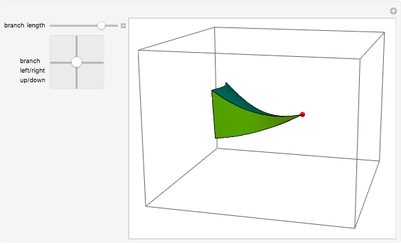
An interactive demonstration that lets the branch and the branch tip around as a function of {?,?}.

Manipulate[
 Graphics3D[{branchOnStem[{{0, 1}, {Pi/2 - 1/2, Pi/2 + 1/2}, 
     1 + ?}, ??],
                          Red, 
   Sphere[branchOnStemEndPoint[{{0, 1}, {Pi/2 - 1/2, Pi/2 + 1/2}, 
      1 + ?}, ??], 0.05]},
   PlotRange -> {{-2, 2}, {0, 4}, {-1, 2}},
  ViewPoint -> {3.17, 0.85, 0.79}],
 {{?, 1.6, "branch length"}, 0, 2, ImageSize -> Small},
 {{??, {0, 0}, 
   "branch\nleft/right\nup/down"}, {-1, -1}, {1, 1}},
 ControlPlacement -> Left, SaveDefinitions -> True]

Adding Branches to a Tree Stem

The stem is just a cone with the cone tip being the tree top.

stem = Cone[{{0, 0, 0}, {0, 0, treeHeight}}, 1];

Branch dimensions decrease with height; getting geometrically smaller. The total of all branch levels equals the tree height minus the step part at the bottom.

heightList1 = 
 Module[{? = 0.8, hs, sol},

  hs = Prepend[Table[C  ?^k, {k, 0, verticalBranchCount - 1}], 
    0];
                 sol = Solve[Total[hs] == 10, C, Reals];
                Accumulate[hs /. sol[[1]]]]

{0, 2.97477, 5.35459, 7.25845, 8.78153, 10.}

treeWidthOfHeight[h_] := treeWidth (treeHeight - h)/treeHeight

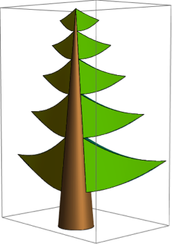
The branches fit snug onto the stem, no gaps in-between.

Graphics3D[{{stemColor, stem}, 
   {Darker[Green], 
   Table[Table[
     branchOnStem[{2 + 
        heightList1[[{j, j + 1}]], {k , k + 1} 2 Pi/
         radialBranchCount , 

       treeWidthOfHeight[Mean[heightList1[[{j, j + 1}]]]]}, {0, 
       0}], {k, 0, 1}] ,
           {j, 1, verticalBranchCount}]}}, 
 ViewPoint -> {2.48, -2.28, 0.28}]

Graphics3D[{{stemColor, stem}, 
   {Darker[Green], 
   Table[Table[
     branchOnStem[{2 + 
        heightList1[[{j, j + 1}]], {k , k + 1} 2 Pi/
         radialBranchCount , 

       treeWidthOfHeight[Mean[heightList1[[{j, j + 1}]]]]}, {0, 
       0}], {k, 0, radialBranchCount - 1}] ,
           {j, 1, verticalBranchCount}]}}, 
 ViewPoint -> {2.48, -2.28, 0.28}]

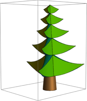
Interleave branches to get a more realistic tree shape. This is the tree I will be using in the following. It is straightforward to change the tree parameters and use another tree.

heightList2 = {2/3, 1/3}.# & /@ Partition[heightList1, 2, 1];

Graphics3D[{{Darker[Brown], stem},
    {EdgeForm[],
     Table[
    Table[branchOnStem[ {2 + 
        heightList1[[{j, j + 1}]], {k , k + 1} 2 Pi/
         radialBranchCount , 

       treeWidthOfHeight[Mean[heightList1[[{j, j + 1}]]]]}, {0, 
       0}], {k, 0, radialBranchCount - 1}] ,
           {j, 1, verticalBranchCount}],
   Table[Table[
     branchOnStem[{2 + 
        heightList2[[{j, j + 1}]], {k , k + 1} 2 Pi/
          radialBranchCount + Pi/radialBranchCount, 

       treeWidthOfHeight[Mean[heightList2[[{j, j + 1}]]]]}, {0, 
       0}], {k, 0, radialBranchCount - 1}] ,
           {j, 1, verticalBranchCount - 1}]}}, 
 ViewPoint -> {2.48, -2.28, 0.28}]

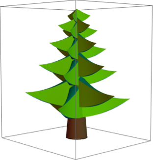
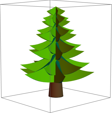
One could easily make even denser trees with more branches.

Graphics3D[{{Darker[Brown], stem},
    {EdgeForm[], 
   Table[Table[branchOnStem[ {2 + heightList1[[{j, j + 1}]],
       {k , k + 1} 2 Pi/(2 radialBranchCount) , 

       treeWidthOfHeight[Mean[heightList1[[{j, j + 1}]]]]}, {0, 
       0}], {k, 0, (2 radialBranchCount) - 1}] ,   {j, 1, 
     verticalBranchCount}],
   Table[Table[branchOnStem[{2 + heightList2[[{j, j + 1}]],
       {k , k + 1} 2 Pi/(2 radialBranchCount) + 
        Pi/(2 radialBranchCount), 

       treeWidthOfHeight[Mean[heightList2[[{j, j + 1}]]]]}, {0, 
       0}], {k, 0, 2 radialBranchCount - 1}] ,
           {j, 1, verticalBranchCount - 1}]}}, 
 ViewPoint -> {2.48, -2.28, 0.28}]

Decorating the Tree

Now let's construct a few ornaments to build a nicely decorated Christmas tree. I all add shiny balls, five-pointed stars and candles. I recommend original Thuringian Lauscha baubles for your Christmas tree. (You can get them here.)

Ornaments, Candles, and the Top

Colored Balls

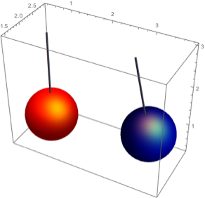
A must on every tree are some shiny glass spheres, baubles.

coloredBall[p_, size_, color_, {?_, ?_}] := 
 Module[{\[ScriptD] = {Cos[?] Sin[?], 
     Sin[?] Sin[?], -Cos[?]}},
  {EdgeForm[], GrayLevel[0.4],  Specularity[Yellow, 20], 
   Cylinder[{p, p + 1.5 size \[ScriptD]}, 0.02 size ],
   color, Specularity[Yellow, 10],
   Sphere[p + (1.5 size + 0.6 size) \[ScriptD] , 0.6 size] 
     }]

Graphics3D[{coloredBall[{1, 2, 3}, 1, Red, {0, 0}], 
  coloredBall[{3, 2, 3}, 1, Darker[Blue], {1, 0.2}]}, Axes -> True]

branchOnStemWithBall[{{hb_, ht_}, {?1_, ?2_}, 
   R_}, {?_, ?_}, color_, {?_, ?_}] := 
 {branchOnStem[{{hb, ht}, {?1, ?2}, 
    R}, {?, ?}] ,  
  coloredBall[
   branchOnStemEndPoint[{{hb, ht}, {?1, ?2}, 
     R}, {?, ?}], 0.45 (ht - hb)/2, 
   color, {?, ?}]}

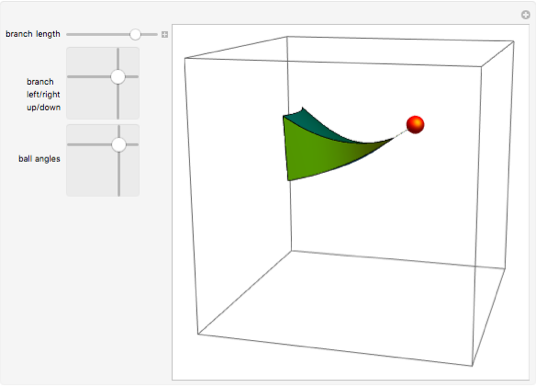
Here is a branch with a bauble. The {?,?} variables allow to change the position of the ball relative to the branch tip.

Manipulate[
 Graphics3D[{branchOnStemWithBall[{{0, 1}, {Pi/2 - 1/2, Pi/2 + 1/2}, 
     1 + ?}, ??, Red, ??]},
   PlotRange -> {{-2, 2}, {0, 4}, {-2, 2}},
  ViewPoint -> {3.17, 0.85, 0.79}],
 {{?, 1.6, "branch length"}, 0, 2, ImageSize -> Small},
 {{??, {0.6, 0.26}, 
   "branch\nleft/right\nup/down"}, {-1, -1}, {1, 1}},
 {{??, {2.57, 1.88}, "ball angles"}, {0, -Pi}, {Pi, Pi}},
 ControlPlacement -> Left, SaveDefinitions -> True]

Here is a tree with balls mostly straight down. I will use random colors for the balls.

Graphics3D[{{Darker[Brown], 
   stem},  {Table[
    Table[branchOnStemWithBall[{2 + 
        heightList1[[{j, j + 1}]], {k , k + 1} 2 Pi/
         radialBranchCount , 

       treeWidthOfHeight[Mean[heightList1[[{j, j + 1}]]]]}, {0, 0},
                              RandomColor[], {0, 0}], {k, 0, 
      radialBranchCount - 1}] ,
           {j, 1, verticalBranchCount}]
   }}, ViewPoint -> {2.48, -2.28, 0.28}, Axes -> True]

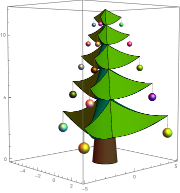
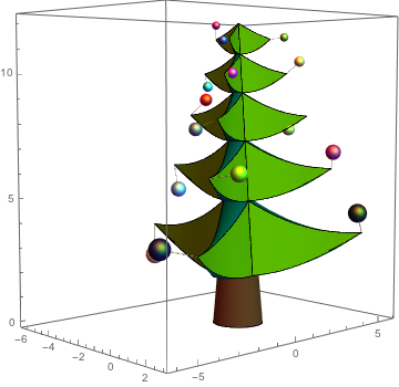
A tree with balls in random directions. If later the branches will be moved, the natural movements (meaning the solution of the corresponding equations of motion) of the balls will be calculated.

Graphics3D[{{Darker[Brown], 
   stem},  {Table[
    Table[branchOnStemWithBall[{2 + 
        heightList1[[{j, j + 1}]], {k , k + 1} 2 Pi/
         radialBranchCount , 

       treeWidthOfHeight[Mean[heightList1[[{j, j + 1}]]]]}, {0, 0},

      RandomColor[], {RandomReal[{-Pi, Pi}], 
       RandomReal[{0, Pi}]}], {k, 0, radialBranchCount - 1}] ,
           {j, 1, verticalBranchCount}]}}, 
 ViewPoint -> {2.48, -2.28, 0.28}, Axes -> True]

Five-pointed Stars

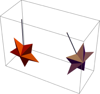
Now some 5-stars. As this ornament is not rotational symmetric, I allow for an orientation angle with respect to the thread it hangs on.

coloredFiveStar[p_, size_, dir_, 
  color_, ?_, {?_, ?_}] := 
 Module[{\[ScriptD] = {Cos[?] Sin[?], 
     Sin[?] Sin[?], -Cos[?]}, points, P1, P2, d1, 
   d2, d3, dP, dP2},
    d2 = Normalize[dir - dir.\[ScriptD] \[ScriptD]]; 
  d3 = Cross[\[ScriptD], d2];
  {EdgeForm[], GrayLevel[0.4], Specularity[Pink, 20],  
   Cylinder[{p, p + (1.5 size + 0.6 size) \[ScriptD]}, 0.02 size ],
   color, Specularity[Hue[.125], 5], 
   dP = Sin[?] d2 + Cos[?] d3;  
   dP2 = Cross[\[ScriptD], dP];
   points = 
    Table[p + (1.5 size + 0.6 size) \[ScriptD]  +   
      size If[EvenQ[j], 1, 1/2] *
                              (Cos[j 2 Pi/10 ] \[ScriptD] + 
         Sin[j 2 Pi/10] dP),   {j, 0, 10}]; 
   P1 = p + (1.5 size + 0.6 size) \[ScriptD] + size/3 dP2;
   P2 = p + (1.5 size + 0.6 size) \[ScriptD] - size/3 dP2; 
   {P1, P2} = (p + (1.5 size + 0.6 size) \[ScriptD]  + #  size/
          3 dP2) & /@ {+1, -1};
   Polygon[
    Join @@ (Function[a, 
        Append[#, a] & /@ Partition[points, 2, 1]] /@ {P1, P2})]
     }]

Graphics3D[{coloredFiveStar[{1, 2, 3}, 0.2, {0, -1, 0}, Darker[Red], 
   0, {0, 0}],

  coloredFiveStar[{1.5, 2, 3}, 0.2, {0, -1, 0}, Darker[Purple], 
   Pi/3, {1, 0.4}]}]

branchOnStemWithFiveStar[{{hb_, ht_}, {?1_, ?2_}, 
   R_}, {?_, ?_}, 
  color_, ?_, {?_, ?_}] := 
 Module[{dir = 
    Append[Normalize[
      Mean[{{Cos[?1], 
         Sin[?1]}, {Cos[?2], 
         Sin[?2]}}]], 0]},
  {branchOnStem[{{hb, ht}, {?1, ?2}, 
     R}, {?, ?}] ,  
   coloredFiveStar[
    branchOnStemEndPoint[{{hb, ht}, {?1, ?2}, 
      R}, {?, ?}], 0.4 (ht - hb)/2, dir, 
    color, ?, {?, ?}]} ]

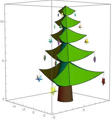
A tree decorated with 5-stars.

Graphics3D[{{Darker[Brown], 
   stem},  {Table[
    Table[branchOnStemWithFiveStar[{2 + 
        heightList1[[{j, j + 1}]], {k , k + 1} 2 Pi/
         radialBranchCount , 

       treeWidthOfHeight[Mean[heightList1[[{j, j + 1}]]]]}, {0, 0},
                              RandomColor[], 
      RandomReal[{-Pi, Pi}], {RandomReal[{-Pi, Pi}], 
       RandomReal[0.1 {-1, 1}]}], {k, 0, radialBranchCount - 1}] ,
           {j, 1, verticalBranchCount}]
   }}, ViewPoint -> {2.48, -2.28, 0.28}, Axes -> True]

Candles

Build from a foot that attaches to the branch tips, a wax-like body, a blackened wick, and a flame. To make like easier for the animation and to avoid fire hazards, I will use electric candles so that the flame will not change shape as the branches move around.

flamePoints = 
 Table[{0.2 Sin[Pi z]^2 Cos[?], 
   0.2 Sin[Pi z]^2 Sin[?], z}, {z, 0, 1, 
   1/1/12}, {?, Pi/2, 5/2 Pi, 2 Pi/24}]

litCandle[p_, size_, color_] := 
 {EdgeForm[], color, 
  Cylinder[{p + {0, 0, size 0.001}, p + {0, 0, size 0.5}}, size  0.04],
  GrayLevel[0.1], Specularity[Orange, 20],
  Cylinder[{p, p + {0, 0, size 0.05}}, size  0.06],
  Black, Glow[Black], 
  Cylinder[{ p + {0, 0, size 0.5}, p + {0, 0, size 0.5 + 0.05 size}}, 
   size 0.008],
  Glow[Orange], Specularity[Hue[.125], 5], 
  BSplineSurface[
   Map[(p + {0, 0, size 0.5} + 0.3 size #) &, flamePoints, {2}],
   SplineClosed -> {True, False}]
    }

A white and a red candle.

Graphics3D[{litCandle[{0, 0, 0}, 1, 
   Directive[White, Glow[GrayLevel[0.3]],  Specularity[Yellow, 20]]], 
  litCandle[{0.5, 0, 0}, 1, 
   Directive[Red, Glow[GrayLevel[0.1]],  Specularity[Yellow, 20]]]}]

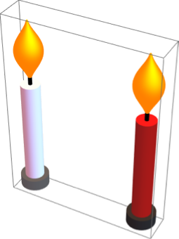
Later, I will use an extended branch with a candle to be the conductor, so I will allow the candle to be tilted away from the stem.

branchOnStemWithCandle[{{hb_, ht_}, {?1_, ?2_}, 
   R_}, {?_, ?_}, color_, ?_] := 
 {branchOnStem[{{hb, ht}, {?1, ?2}, 
    R}, {?, ?}] ,  
  If[? == 0, 
   litCandle[
    branchOnStemEndPoint[{{hb, ht}, {?1, ?2}, 
      0.98 R}, {?, ?}], 0.66 (ht - hb) , color],
   Module[{P = 
      branchOnStemEndPoint[{{hb, ht}, {?1, ?2}, 
        0.98 R}, {?, ?}], dir},
    dir = Append[Reverse[Take[P, 2]] {-1, 1}, 0];
    Rotate[
     litCandle[
      branchOnStemEndPoint[{{hb, ht}, {?1, ?2}, 
        0.98 R}, {?, ?}], 0.66 (ht - hb) , 
      color], ?, dir, P]]]}

Manipulate[
 Graphics3D[{branchOnStemWithCandle[{{0, 1}, {Pi/2 - 1/2, Pi/2 + 1/2},
      1 + ?}, ??, Red, ?]},
   PlotRange -> {{-2, 2}, {0, 4}, {-2, 2}},
  ViewPoint -> {3.17, 0.85, 0.79}],
 {{?, 1.6, "branch length"}, 0, 2, ImageSize -> Small},
 {{??, {0, 0}, 
   "branch\nleft/right\nup/down"}, {-1, -1}, {1, 1}},
 {{?, Pi/4, "candle angle"}, -Pi, Pi},
 ControlPlacement -> Left, SaveDefinitions -> True]

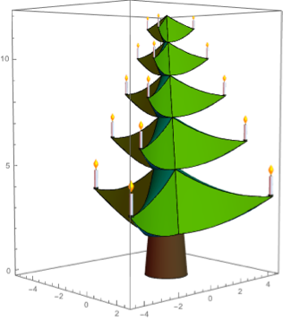
And here is a tree with a candle on each branch.

Graphics3D[{{Darker[Brown], 
   stem},  {Table[
    Table[branchOnStemWithCandle[{2 + 
        heightList1[[{j, j + 1}]], {k , k + 1} 2 Pi/
         radialBranchCount , 
        treeWidthOfHeight[Mean[heightList1[[{j, j + 1}]]]]}, {0, 0},
                              White, 0], {k, 0, 
      radialBranchCount - 1}] ,
           {j, 1, verticalBranchCount}]
   }}, ViewPoint -> {2.48, -2.28, 0.28}, Axes -> True]

Tree Topper

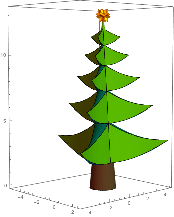
For fun, I add a rotatable spikey at the top.

spikey = Cases[
    N@Entity["Polyhedron", "RhombicHexecontahedron"][
      "Image"], _GraphicsComplex, ?][[1]];

top = {Gray, Specularity[Red, 25], 
  Cone[{{0, 0, 0.9 treeHeight}, {0, 0, 1.08 treeHeight}}, 
   treeWidth/240],
         Orange, EdgeForm[Darker[Orange]], Specularity[Hue[.125], 5],

  MapAt[((0.24 # + {0, 0, 1.08 treeHeight}) & /@ #) &, spikey, 1]
  }
Graphics3D[{{Darker[Brown], stem}, 
   {Table[
    Table[branchOnStem[{2 + 
        heightList1[[{j, j + 1}]], {k , k + 1} 2 Pi/
         radialBranchCount , 

       treeWidthOfHeight[Mean[heightList1[[{j, j + 1}]]]]}, {0, 
       0} ], {k, 0, radialBranchCount - 1}] ,
           {j, 1, verticalBranchCount}],
   top}}, ViewPoint -> {2.48, -2.28, 0.28}, Axes -> True]

Decorating the Tree

We will single out a single branch as the conductor. The remaining branches we will randomly divide into four groups and decorate them with baubles of two colors, five-pointed stars, and candles.

Now let's add an ornament or a candle on every tree branch. I will use the above tree with 27 branches. I start the branches by height on the stem and by azimuthal angle.

allBranches = 
 Flatten[Riffle[
   Table[Table[{2 + 
       heightList1[[{j, j + 1}]], {k , k + 1} 2. Pi/
        radialBranchCount , 

      treeWidthOfHeight[Mean[heightList1[[{j, j + 1}]]]]}, {k, 0, 
      radialBranchCount - 1}] ,
           {j, 1, verticalBranchCount}],
   Table[Table[{2 + 
       heightList2[[{j, j + 1}]], {k , k + 1} 2. Pi/
         radialBranchCount + Pi/radialBranchCount, 

      treeWidthOfHeight[Mean[heightList2[[{j, j + 1}]]]]}, {k, 0, 
      radialBranchCount - 1}] ,
           {j, 1, verticalBranchCount - 1}]], 1]

Length[allBranches]

27

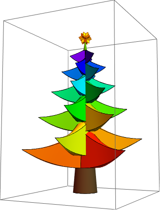
Color branches by index, starting at the bottom in red to the top in purple.

Graphics3D[{{Darker[Brown], stem},
  MapIndexed[(branchOnStem[#1, {0, 0}] /. _RGBColor :> 
       Hue[#2[[1]]/36]) &, allBranches],
  top}, ViewPoint -> {2, 1, -0.2}]

Split all branches into 4 groups for the voices and a conductor branch.

conductorBranch = 7;

SeedRandom[12];
voiceBranches = (Last /@ #) & /@ 
  GroupBy[{RandomChoice[{1, 2, 3, 4}], #} & /@ 
    Delete[Range[27], {conductorBranch}], First]

<|1 -> {1, 4, 5, 6, 12, 18, 20}, 3 -> {2, 8, 10, 11, 14, 22, 23, 25}, 2 -> {3, 13, 15, 16, 21, 26}, 4 -> {9, 17, 19, 24, 27}|>

voiceBranches = <|1 -> {2, 9, 14, 17, 19, 24, 27}, 
  2 -> {3, 13, 15, 16, 21, 26}, 3 -> {1, 4, 5, 12, 18, 20}, 
  4 -> {6, 8, 10, 11, 22, 23, 25}|>

<|1 -> {2, 9, 14, 17, 19, 24, 27}, 2 -> {3, 13, 15, 16, 21, 26}, 3 -> {1, 4, 5, 12, 18, 20}, 4 -> {6, 8, 10, 11, 22, 23, 25}|>

Here is a plot of the branches colored according to which voice they represent.

Graphics3D[{{Darker[Brown], stem},
  branchOnStem[#1, {0, 0}] & /@ 
    allBranches[[voiceBranches[[1]]]] /. _RGBColor :> Yellow,
  branchOnStem[#1, {0, 0}] & /@ 
    allBranches[[voiceBranches[[2]]]] /. _RGBColor :> White,
  branchOnStem[#1, {0, 0}] & /@ 
    allBranches[[voiceBranches[[3]]]] /. _RGBColor :> LightBlue,
  branchOnStem[#1, {0, 0}] & /@ 
    allBranches[[voiceBranches[[4]]]] /. _RGBColor :> Pink,
  branchOnStem[
    allBranches[[conductorBranch]] {1, 1, 1.5}, {0, 
     0}] /. _RGBColor :> Red,
  top}, ViewPoint -> {2, 1, -0.2}]

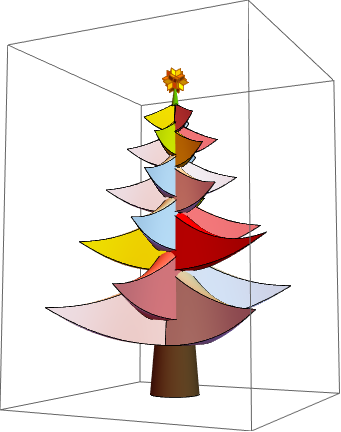
The final tree with the branch tip positions as parameters. Also allow the ornaments on the branch tips angled and colored.

christmasTree[{{?1_, ?1_}, {?2_, ?2_}, {?3_, ?3_}, {?4_, ?4_}, {?c_, ?c_}}, 
                            {{?1_, ?1_}, {?2_, ?2_}, {?3_, ?3_}},  
                             {colBall1_, colBall2_, col5Star_},
                           conductorEnhancementFactor : fc_, 
                           conductorCandleAngle : ?c_, topRotationAngle : ?_] := 
  {{Darker[Brown], stem}, 
   branchOnStemWithBall[#, {?1, ?1}, 
      colBall1, {?1, ?1}] & /@ 
    allBranches[[voiceBranches[[1]]]],
   branchOnStemWithBall[#, {?2, ?2}, 
      colBall2, {?2, ?2}] & /@ 
    allBranches[[voiceBranches[[2]]]],
   branchOnStemWithFiveStar[#, {?3, ?3}, col5Star, 
      Pi/4, {?3, ?3}] & /@ 
    allBranches[[voiceBranches[[3]]]], 
   branchOnStemWithCandle[#, {?4, ?4}, 
      Directive[White, Glow[GrayLevel[0.3]], Specularity[Yellow, 20]],
       0] & /@ allBranches[[voiceBranches[[4]]]],
   branchOnStemWithCandle[
    allBranches[[conductorBranch]] {1, 1, 
      1 + fc}, {?c, ?c}, 
    Directive[Red, Glow[GrayLevel[0.1]],  
     Specularity[Yellow, 20]], ?c],
   Rotate[top, ?, {0, 0, 1}]
   };

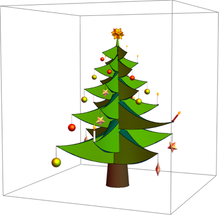
Resting position of all branches and the conductor branch elongated and its candle angled.

Graphics3D[christmasTree[{{0, 0}, {0, 0}, {0, 0}, {0, 0}, {0, 0}},
                                                          {{0, 0}, {0,0}, {0, 0}}, {Red, Darker[Yellow], Pink}, 0.8, Pi/4, 0], 
 ImageSize -> 600, ViewPoint -> {3.06, 1.28, 0.27},  
 PlotRange -> {{-7, 7}, {-7, 7}, {0, 15}}]

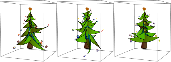
Three trees with all parameters selected randomly.

SeedRandom[1]
Table[Graphics3D[christmasTree[RandomReal[1.5 {-1, 1}, {5, 2}],

    Table[{RandomReal[{-Pi, Pi}], RandomReal[{0, Pi}]}, 3],
                                            RandomColor[3], 
    RandomReal[], RandomReal[Pi/2], 0], ImageSize -> 200, 
   ViewPoint -> {3.06, 1.28, 0.27},  
   PlotRange -> {{-7, 7}, {-7, 7}, {-2, 15}}], {3}] // Row

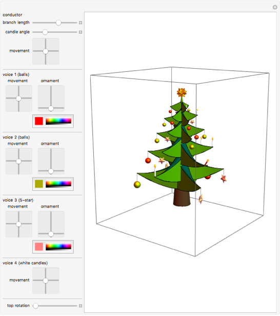
The following interactive demonstrations allows to move the branches, move ornaments around with respect to the branch tips and to color the ornaments to ones personal preferences.

Manipulate[
 Graphics3D[
  christmasTree[{??1, ??2, ??3, ??4, ??c}, 
                                                         {??1, ??2, ??3}, {col1, col2, col3}, 
   l, ?c, ?],
                           ImageSize -> 400, 
  ViewPoint -> {2.61, 1.99, 0.80},

  PlotRange -> {{-7, 7}, {-7, 7}, {-2, 15}}],
 "conductor",
 {{l, 0.6, "branch length"}, 0, 1, ImageSize -> Small},
 {{?c, Pi/4, "candle angle"}, 0, Pi, ImageSize -> Small},
 {{??c, {0, 0}, "movement"}, {-1, -1}, {1, 1}, 
  ImageSize -> Small},
 Delimiter,
 "voice 1 (balls)",
 Grid[{{"movement", "ornament"},
   {Control[{{??1, {0, 0}, ""}, {-1, -1}, {1, 1}, 
      ImageSize -> Small}],
    Control[{{??1, {0, 0}, ""}, {-Pi, 0}, {Pi, Pi}, 
      ImageSize -> Small}]}}],
 {{col1, Red, ""}, Red, ImageSize -> Tiny},
 Delimiter,
 "voice 2 (balls)",
 Grid[{{"movement", "ornament"},
   {Control[{{??2, {0, 0}, ""}, {-1, -1}, {1, 1}, 
      ImageSize -> Small}],
    Control[{{??2, {0, 0}, ""}, {-Pi, 0}, {Pi, Pi}, 
      ImageSize -> Small}]}}],
 {{col2, Darker[Yellow], ""}, Red, ImageSize -> Tiny},
 Delimiter,
 "voice 3 (5-star)",
 Grid[{{"movement", "ornament"},
   {Control[{{??3, {0, 0}, ""}, {-1, -1}, {1, 1}, 
      ImageSize -> Small}],
    Control[{{??3, {0, 0}, ""}, {-Pi, 0}, {Pi, Pi}, 
      ImageSize -> Small}]}}],
 {{col3, Pink, ""}, Red, ImageSize -> Tiny},
 Delimiter,
 "voice 4 (white candles)",
  Control[{{??4, {0, 0}, "movement"}, {-1, -1}, {1, 1}, 
   ImageSize -> Small}],
 Delimiter,
  Delimiter,
 {{?, 0, "top rotation"}, 0, 1, ImageSize -> Small},
 ControlPlacement -> Left, SaveDefinitions -> True]

From Music to Movements

So, now that I have dealt with the making a parametrized decorated Christmas tree with movable branches and ornaments, I must deal with relating the music to the movements of the branches (and in turn the ornaments).

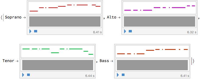
Get the 4 Voices as Sound

Use a MIDI file of the song.

{ohTannenBaum // Head, ohTannenBaum // ByteCount}

{Sound, 287816}

Extract the 4 voices.

voices = AssociationThread[{"Soprano", "Alto", "Tenor", "Bass"}, 
   ImportString[
    ExportString[ohTannenBaum, "MIDI"], {"MIDI", "SoundNotes"}]];

Sound[Take[#, 10]] & /@ voices

Voices to Frequencies

frequencyRules = <|"A1" -> 55., "A2" -> 110., "A3" -> 220., 
   "A4" -> 440., "B1" -> 61.74, "B2" -> 123.5, "B3" -> 246.9, 
   "B4" -> 493.9, "C2" -> 65.41, "C3" -> 130.8, "C4" -> 261.6, 
   "C5" -> 523.3, "D2" -> 73.42, "D#4" -> 311.13, "D4" -> 293.7, 
   "D5" -> 587.3, "E2" -> 82.41, "E4" -> 329.6, "E5" -> 659.3, 
   "F#2" -> 92.50, "F#4" -> 370.0, "G2" -> 98.00, "G#4" -> 415.3, 
   "G4" -> 392.0|>;

{minf, maxf} = MinMax[frequencyRules]

{55., 659.3}

Time-frequency plot of the first voice.

pw[t_] = Piecewise[{frequencyRules[#1], #2[[1]] <= t <= #2[[2]]} & @@@
     voices[[1]]];
Plot[pw[t], {t, 0, 100}, PlotRange -> {200, All}, Filling -> Axis, 
 PlotLabel -> "Soprano",
 Frame -> True, FrameLabel -> {"time in sec", "frequency in Hz"}, 
 AxesOrigin -> {0, 200}]

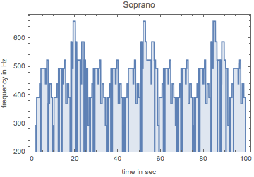
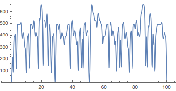
For representing the frequencies in the movements, I will smooth the curves.

spline = BSplineFunction[Table[{t, pw[t]}, {t, 0, 100, 0.5}], 
  SplineDegree -> 2]

ParametricPlot[spline[t], {t, 0, 100}, AspectRatio -> 0.5, 
 PlotPoints -> 1000]

tMax = 100;
Do[
 With[{j = j},
  pwf[j][t_] = 
   Piecewise[{frequencyRules[#1], #2[[1]] <= t <= #2[[2]]} & @@@ 
     voices[[j]]];
  splineFunction[j] = 
   BSplineFunction[Table[{t, pwf[j][t]}, {t, 0, 100, 0.5}], 
    SplineDegree -> 2];
  voiceFunction[j][t_Real] := 
   If[0 < t < tMax, splineFunction[j][t/tMax][[2]]/maxf, 0]],
 {j, 4}]

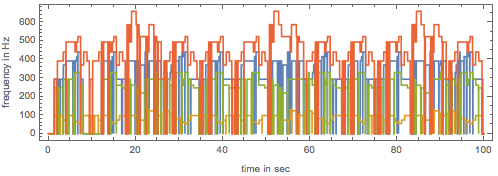
The frequencies of the four voices.

Plot[Evaluate[Reverse@Table[pwf[j][t], {j, 4}]], {t, 0, 100}, 
 Frame -> True, FrameLabel -> {"time in sec", "frequency in Hz"}, 
 AspectRatio -> 0.3]

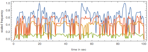
Smoothed scaled frequencies of the four voices.

Plot[Evaluate[Table[voiceFunction[j][t], {j, 4}]], {t, 0, 100}, 
 Frame -> True, FrameLabel -> {"time in sec", "scaled frequency"}, 
 AspectRatio -> 0.3]

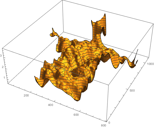
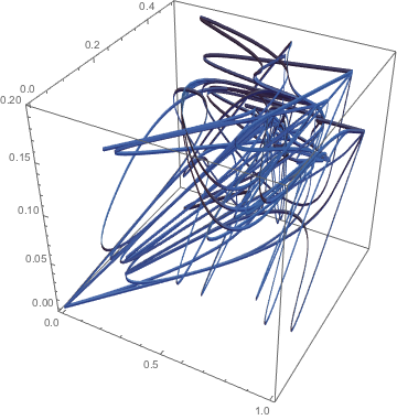
Here is a plot of the (smoothed) first three voices as a 3D plot.

ParametricPlot3D[{voiceFunction[1][t], voiceFunction[2][t], 
  voiceFunction[3][t]}, {t, 0, 100}, AspectRatio -> Automatic, 
 PlotPoints -> 1000, BoxRatios -> {1, 1, 1}]

Show[% /. Line[pts_] :> Tube[pts, 0.002], 
 Method -> {"TubePoints" -> 4}]

Get Sway Pattern

Anchor to particular phrases to generate all measure beats.

{firstBeat, secondBeat, lastBeat} = 
 voices["Soprano"][[{1, 2, -1}, 2, 1]]

{1.33522, 2.00568, 98.7727}

    anchorDataOChristmasTree = SequenceCases[
       voices["Soprano"],
       (* pattern for "O Christmas Tree, O Christmas Tree..." *)
       {
         SoundNote["D4", {pickupStart_, _}, "Trumpet", ___],
         SoundNote["G4", {beatOne_, _}, "Trumpet", ___],
         SoundNote["G4", {_, _}, "Trumpet", ___],
         SoundNote["G4", {beatTwo_, _}, "Trumpet", ___],
         SoundNote["A4", {beatThree_, _}, "Trumpet", ___],
         SoundNote["B4", {beatFour_, _}, "Trumpet", ___],
         SoundNote["B4", {_, _}, "Trumpet", ___],
         SoundNote["B4", {beatFive_, _}, "Trumpet", ___]
         } :> <|
         "PhraseName" -> "O Christmas Tree",
         "PickupBeat" -> pickupStart,
         "TargetMeasureBeats" -> {beatOne, beatTwo, beatThree},
         "BeatLength" -> 
          Mean@Differences[{pickupStart, beatOne, beatTwo, beatThree, 
             beatFour, beatFive}]
         |>
       ];

anchorDataYourBoughsSoGreen = SequenceCases[
   voices["Soprano"],
   (* "Your boughs so green in summertime..." *)
   {
     SoundNote["D5", {pickupBeatAnd_, _}, "Trumpet", ___],
     SoundNote["D5", {beatOne_, _}, "Trumpet", ___],
     SoundNote["B4", {_, _}, "Trumpet", ___],
     SoundNote["E5", {beatTwo_, _}, "Trumpet", ___],
     SoundNote["D5", {beatThreeAnd_, _}, "Trumpet", ___],
     SoundNote["D5", {beatFour_, _}, "Trumpet", ___],
     SoundNote["C5", {_, _}, "Trumpet", ___],
     SoundNote["C5", {beatFive_, _}, "Trumpet", ___]
     } :> With[
     {
      (* the offbeat nature of this phrase requires some manual work 
         to get things lined up in terms of actual beats *)

      pickupBeatStart = pickupBeatAnd - (beatOne - pickupBeatAnd),
      beatThree = beatThreeAnd - (beatFour - beatThreeAnd)
      },
     <|
      "PhraseName" -> "Your boughs so green in summertime",
      "PickupBeat" -> pickupBeatStart,
      "TargetMeasureBeats" -> {beatOne, beatTwo, beatThree},
      "BeatLength" -> 
       Mean@Differences[{pickupBeatStart, beatOne, beatTwo, beatThree,
           beatFour, beatFive}]
      |>
     ]
   ];

anchorData0 = 
  Join[anchorDataOChristmasTree, anchorDataYourBoughsSoGreen] // 
   SortBy[#PickupBeat &];
meanBeatLength = Mean[anchorData0[[All, "BeatLength"]]];

(* add enough beats to fill the end of the song, which ends on beat 2 *)
anchorData = 
  Append[anchorData0, <|
    "TargetMeasureBeats" -> (lastBeat + {-1, 0, 1}*
        Last[anchorData0]["BeatLength"]), 
    "BeatLength" -> Last[anchorData0]["BeatLength"]|>];
anchorData = 
  Append[anchorData, <|
    "TargetMeasureBeats" -> (lastBeat + ({-1, 0, 1} + 3)*
        Last[anchorData]["BeatLength"]), 
    "BeatLength" -> Last[anchorData]["BeatLength"]|>];

Interpolate the beats between and during phrases:

interpolateAnchor = Apply[
   Function[{currentAnchor, nextAnchor},
    With[
     {targetMeasureLastBeat = 
       Last[currentAnchor["TargetMeasureBeats"]],
      nextMeasureFirstBeat = 
       First[nextAnchor["TargetMeasureBeats"]]},
     DeleteDuplicates@Join[
       currentAnchor["TargetMeasureBeats"],
       Range[targetMeasureLastBeat, 
        nextMeasureFirstBeat - currentAnchor["BeatLength"]/4., 
        Mean[{currentAnchor["BeatLength"], nextAnchor["BeatLength"]}]]]
     ]]];

measureBeats = Flatten@BlockMap[interpolateAnchor, anchorData, 2, 1];
measureBeats // Length

144

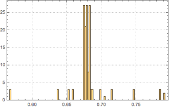
The beats vary slightly, which, if not taken into account with the anchoring method above, can cause phasing between the motion and the sound:

Histogram[Differences[measureBeats], PlotTheme -> "Detailed", PlotRange -> Full]

    (* add pickup beat at start *)

    swayControlPoints = 
      Prepend[Join @@ (Partition[measureBeats, 3, 3, 1, {}] //

          MapIndexed[
           Function[{times, index}, {#, (-1)^(Mod[index[[1]], 2] + 1)} & /@
              times]]), {firstBeat, -1}];

swayControlPointPlot = 
  ListPlot[swayControlPoints, Joined -> True, Mesh -> All, 
   AspectRatio -> 1/6, PlotStyle ->
    {Darker[Purple]}, PlotTheme -> "Detailed", 
   MeshStyle -> PointSize[0.008], ImageSize -> 600, 
   Epilog -> {Darker[Green], Thick, 
     InfiniteLine[{{#, -1}, {#, 1}}] & /@ {firstBeat, secondBeat, 
       lastBeat}}];

sway = BSplineFunction[
   Join[{{0, 0}}, 
    Select[swayControlPoints, #[[1]] < tMax &], {{100, 0}}], 
   SplineDegree -> 3];

sh = Show[{swayControlPointPlot, 
   ParametricPlot[sway[t], {t, 0, tMax}, PlotPoints -> 2500]}]

{Show[sh, PlotRange -> {{0, 10}, All}], Show[sh, PlotRange -> {{90, 105}, All}]}

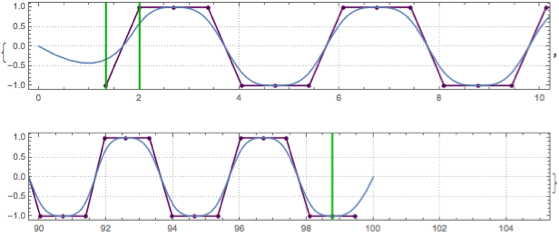
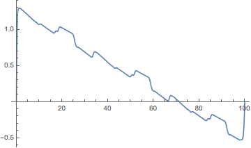
Now, a subtle point: Interpolating with B-splines gives nice smooth curves. In distinction to Interpolation, the actual given points are not on the resulting curve. This looks nice and smooth and is what we want for visual purposes of this animation. But the interpolation is for the pair of points. This means that for a given argument (between 0 and 1) of the B-spline function, ones does not get a linear interpolation with respect to the first argument. Rather, one has to invert the interpolation to get time as a function of the interpolation parameter variable. Taking this effect into account is important to properly align the music with the branch movements.

swayTimeCoordinate = Interpolation[Table[{t, sway[t/100][[1]]}, {t, 0, 100, 0.1}],  InterpolationOrder -> 1]

This plot shows the difference between the interpolation and the rescaled B-spline function parameter.

Plot[swayTimeCoordinate[t] - t, {t, 0, 100}]

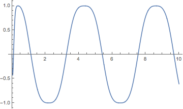
swayOfTime[t_] := sway[swayTimeCoordinate[t]/100][[2]]

Plot[swayOfTime[t], {t, 0, 10}]

Visualize the phrases and how they relate to the sway motion with Tooltip and colored rectangles:

phraseGraphics = BlockMap[
   Apply[
    Function[{currentAnchor, nextAnchor},
     With[
      {phraseStart = currentAnchor["PickupBeat"],
       phraseEnd = 
        nextAnchor["PickupBeat"] - currentAnchor["BeatLength"]},
      {Switch[currentAnchor["PhraseName"],
        "O Christmas Tree", Opacity[0.25, Gray],
        "Your boughs so green in summertime", 
        Opacity[0.25, Darker@Green],
        _, Black],
       Tooltip[
        Polygon[
         {{phraseStart, -10}, {phraseStart, 10}, {phraseEnd, 
           10}, {phraseEnd, -10}}],
        Grid[{{currentAnchor["PhraseName"], SpanFromLeft},
          {"Phrase Start:", phraseStart}, {"Phrase End:", phraseEnd}
          }]]}]]],
   Append[anchorData0, <|"PickupBeat" -> lastBeat + meanBeatLength|>],
    2, 1];

Show[swayControlPointPlot, 
 ParametricPlot[sway[t], {t, 0, Last[measureBeats]}, 
  ImageSize -> Full, PlotPoints -> 800, AspectRatio -> 1/8, 
  PlotTheme -> "Detailed", PlotRangePadding -> Scaled[.02]], 
 Prolog -> phraseGraphics]

Conductor Movements

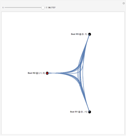
The conductor branch carries out a simple periodic movement that is synchronized to the music.

threePatternPoints = {{0, -1}, {-1, -0}, {0, 1}};
threePatternBackground = ListPlot[
   MapIndexed[
    Callout[#1, StringTemplate["Beat #`` @ ``"][First@#2, #1], Left] &,
    threePatternPoints],
   PlotTheme -> "Minimal", Axes -> False, AspectRatio -> 1,
   PlotStyle -> Directive[Black, PointSize[0.025]],
   PlotRange -> {{-2, 0.75}, {-1.5, 1.5}}];

conductorControlTimes = swayControlPoints[[All, 1]];

(* basic conductor control points for interpolation *)
conductorControlPoints = 
  MapIndexed[{conductorControlTimes[[First[#2]]], #1} &, 
   Join @@ ConstantArray[RotateRight[threePatternPoints, 1], 
     Floor@(Length[conductorControlTimes]/3)]]; 

(* the shape is okay, but not perfect *)

conductor = Interpolation[conductorControlPoints];

(* adding pauses before/after the beat improves the shape of the 
   curves and makes the beats more obvious *)
conductorControlPointsWithPauses = 
  Join @@
   ({# - {meanBeatLength/8., -0.15*
          Normalize[
           Mean[threePatternPoints] - #[[
             2]]]}, #, # + {meanBeatLength/8., 
         0.15*Normalize[
           Mean[threePatternPoints] - #[[
             2]]]}} & /@

     conductorControlPoints); 

This time, I use Interpolation.

conductorWithPauses = 
  Interpolation[conductorControlPointsWithPauses, 
   InterpolationOrder -> 5];

Here is the resulting shape of the baton.

Manipulate[
 Show[threePatternBackground, 
  ParametricPlot[
   conductorWithPauses[t], {t, 
    Max[firstBeat,(*tmax-2*meanBeatLength*)0], tmax},
   PerformanceGoal -> "Quality"], 
  Epilog -> {Red, PointSize[Large], Point[conductorWithPauses[tmax]]},
   ImageSize -> Large], {{tmax, lastBeat, "t"}, firstBeat + 0.0001, 
  lastBeat, Appearance -> "Labeled"},
 SaveDefinitions -> True]

Branch Movements from the Voices

There are various ways how the sound could be 'translated' into movements of the branches. We will give two possibilities, one related to the frequency of the sounds, and another based on the onset of the notes.

Possibility 1

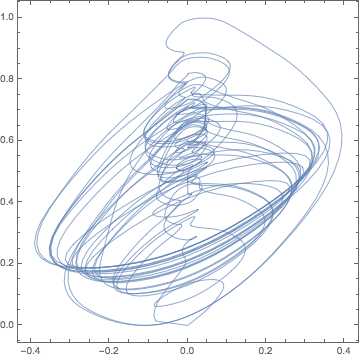
First translation from voice to 2d movements: vertical movement: smoothed frequency of the voice horizontal movement: difference of current smoothed frequency of the voice to slightly earlier frequency

?Delay = 0.3;

voice??[j_][time_] := 
 If[0 < time < tMax,(* smoothing factor *) 
  Sin[Pi time/tMax]^0.25 {voiceFunction[j][1. time] - 
     voiceFunction[j][time - ?Delay],
    voiceFunction[j][1. time]}, {0, 0}]

ParametricPlot[voice??[1][t], {t, 0, tMax}, 
 AspectRatio -> 1, PlotRange -> All, Frame -> True, Axes -> False,
 PlotStyle -> Thickness[0.002]]

Possibility 2

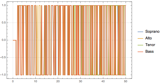
First translation from voice to 2d movements: vertical movement: note changes horizontal movement: sway

 value = -1;
interpolateDance[{{t1_, t2_}, {t3_, t4_}}, t_] :=

  With[{y1 = value, y2 = value = -value},
   {{y1, t1 < t < t2}, {((y1 - y2) t - (t3 y1 - t2 y2))/(t2 - t3), 
     t2 < t < t3}}];

dancingPositionPiecewise[notes : {__SoundNote}] := 
  With[{noteTimes = 
     Cases[notes, 
      SoundNote[_, times : {startTime_, endTime_}, ___] :> times]},
   value = -1;
   Quiet[Piecewise[
     DeleteDuplicatesBy[
      Join @@ BlockMap[interpolateDance[#, t] &, noteTimes, 2, 1], 
      Last], 0]
    ]];

tEnd = Max[voices[[All, All, 2]]];
dancingPositions = dancingPositionPiecewise /@ voices;

Plot[Evaluate[KeyValueMap[Legended[#2, #1] &, dancingPositions]], {t, 
  0, 50},
 PlotRangePadding -> Scaled[.05], PlotRange -> {All, {-1, 1}}, 
 ImageSize -> Large, PlotTheme -> "Detailed", PlotLegends -> None]

dancingPositionPiecewiseList = Normal[dancingPositions][[All, 2]];

bsp = BSplineFunction[
  Table[Evaluate[{t, dancingPositionPiecewiseList[[2]]}], {t, 0, 100, 
    0.2}]]

ParametricPlot[bsp[t], {t, 0, 1}, AspectRatio -> 1/4, 
 PlotPoints -> 2000]

Do[voiceIF[j] = 
  BSplineFunction[
   Table[Evaluate[{t, dancingPositionPiecewiseList[[j]]}], {t, 0, 100,
      0.2}]],
 {j, 4}]

Do[With[{j = j},
  voiceTimeCoordinate[j] = 
   Interpolation[Table[{t, voiceIF[j][t/100][[1]]}, {t, 0, 100, 0.1}],
     InterpolationOrder -> 1]],
 {j, 4}]

The final movements of the branch tips with the ?-? square [-1,1]*[-1,1].

Clear[voice??];
voice??[j_][time_] := 
 If[0 < time < tMax,(* smoothing factor *) Sin[Pi time/tMax]^0.25*
   {sway[swayTimeCoordinate[time]/tMax][[2]], 
    voiceIF[j][voiceTimeCoordinate[j][time]/tMax][[2]]}, {0, 0}]

Table[ListPlot[Table[ voice??[j][t], {t, 0, 105, 0.01}], 
  Joined -> True, AspectRatio -> 1, 
  PlotStyle -> Thickness[0.002]], {j, 4}]

Model the Ornament Swings

Now it is time (finally) to do some physics. The ornaments (ball, five-star) I will model as a forced spherical pendulum with fraction. The forcing is realized through the position of branch tips, which in turn comes from the voice??[j][time].

Forced Spherical Pendulum

Form Lagrangian of a forced spherical pendulum in spherical coordinates.

Clear[r, ?, R, X, Y, Z]
R[t_] := {X[t], Y[t], Z[t]}
r[t_] := R[t] + 
  L {Cos[?[t]] Sin[?[t]], 
    Sin[?[t]] Sin[?[t]], -Cos[?[t]]}
? = 1/2 r'[t].r'[t] - g r[t][[3]]

-g (-L Cos[?[t]] + Z[t]) + 1/2 ((Derivative[1][Z][t] + L Sin[?[t]] Derivative[1][?][t])^2 + (Derivative[ 1][Y][t] + L Cos[?[t]] Sin[?[t]] Derivative[1][?][t] + L Cos[?[t]] Sin[?[t]] Derivative[1][?][ t])^2 + (Derivative[1][X][t] + L Cos[?[t]] Cos[?[t]] Derivative[1][?][t] - L Sin[?[t]] Sin[?[t]] Derivative[1][?][t])^2)

Add a Rayleigh dissipation function ? to account for friction.

? = 1/2 (\[ScriptF]? ?'[t]^2 + \[ScriptF]?  ?'[t]^2);

eoms = {D[D[?, ?'[t]], t] - 
D[?, ?[t]] == -D[?, ?'[t]],

D[D[?, ?'[t]], t] - 
D[?, ?[t]] == -D[?, ?'[
t]]} // Simplify

{([ScriptF]? + L^2 Sin[2 ?[t]] Derivative[1][?][t]) Derivative[ 1][?][t] + L Sin[?[t]] (-Sin?[t]t] + Cos[?[t][t] + L Sin?[t][t]) == 0, [ScriptF]? Derivative[1][?][t] + L (g Sin[?[t]] - L Cos[?[t]] Sin[?[t]] Derivative[1][?][t]^2 + Cos[?[t]] Cos?[t]t] + Cos[?[t]] Sin[?[t]t] + Sin[?[t][t] + L (?^??)[t]) == 0}

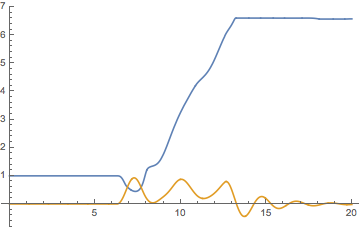
Example showing that the oscillations die out quickly with appropriate parameter values of [ScriptF]?, [ScriptF]?.

 paramRules = { g -> 10, 
   L -> 1, \[ScriptF]? -> 1, \[ScriptF]? -> 1};

In[126]:= X[t_] := If[2 Pi < t < 4 Pi, 8 Cos[t], 8];
Y[t_] := If[2 Pi < t < 4 Pi, 4 Sin[t], 0];
Z[t_] := 0; 

nds = NDSolve[{eoms /. paramRules, ?[0] == 1, ?'[0] == 
    0, ?[0] == 0.001, ?'[0] == 0},
  {?, ?}, {t, 0, 20}, PrecisionGoal -> 3, AccuracyGoal -> 3] 

Plot[Evaluate[{\[Phi][t], \[Theta][t]} /. nds[[1]]], {t, 0, 
  nds[[1, 2, 2, 1, 1, 2]]}, PlotRange -> All]

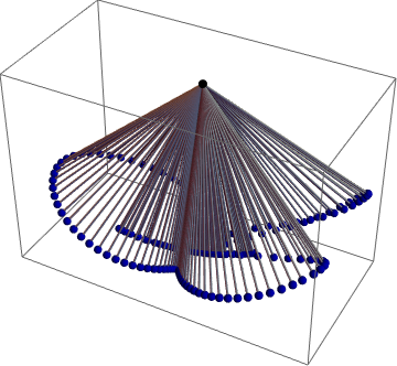
Graphics3D[
 Table[With[{P = r[t] - R[t] /. nds[[1]] /. paramRules}, {Black, 
    Sphere[{0, 0, 0}, 0.02], Gray, Cylinder[{{0, 0, 0}, P}, 0.005],
    Darker[Blue], Sphere[P, 0.02]}],
  {t, 0, 20, 0.05}], PlotRange -> All]

Calculate Ornament Movements

Get the ? and ? direction of the branch tip positions interpolated as a function of time.

branchToVoice = 
 Association[
  Flatten[Function[{v, bs}, (# -> v) & /@  bs] @@@ 
    Normal[voiceBranches]]]

<|2 -> 1, 9 -> 1, 14 -> 1, 17 -> 1, 19 -> 1, 24 -> 1, 27 -> 1, 3 -> 2, 13 -> 2, 15 -> 2, 16 -> 2, 21 -> 2, 26 -> 2, 1 -> 3, 4 -> 3, 5 -> 3,
12 -> 3, 18 -> 3, 20 -> 3, 6 -> 4, 8 -> 4, 10 -> 4, 11 -> 4, 22 -> 4, 23 -> 4, 25 -> 4|>

tValues = Table[1. t , {t, -5, 110, 0.1}];
Do[??Values = 
  Table[voice??[j][t] , {t, -5, 110, 0.1}];
 if?[j] = 
  Interpolation[
   Transpose[{tValues, ??Values[[All, 1]]}]];
 if?[j] = 
  Interpolation[
   Transpose[{tValues, ??Values[[All, 2]]}]],
 {j, 4}]

Calculate the movement of the ornaments modeled as spherical pendula. To get some variation in the movements, I use small random deviations from the vertical as initial conditions for the ornaments (modeling some random thermal air movements).

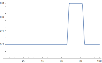
For a time range in the second half, I use a different amplitude (corresponding to louder music) for the forcing amplitudes.

changeTimeList = {17.6, 42.2, 66.8, 83.1};

loudness[t_] :=

 With[{?1 = 0.2, ?2 = 0.8, ?t = 1.5},
   Which[t <= changeTimeList[[3]] - ?t, ?1,
        changeTimeList[[3]] - ?t <= t <= 
    changeTimeList[[3]] + ?t, 
               ?1 + (?2 - 
       1 ?1) (1 - 
        Cos[Pi (t - (changeTimeList[[
                3]] - ?t))/(2 ?t)])/2,

   changeTimeList[[3]] + ?t <= t <=  
    changeTimeList[[4]] - ?t , ?2,

   changeTimeList[[4]] - ?t <= t <= 
    changeTimeList[[4]] + ?t,
               ?1 + (?2 - 
       1 ?1) (1 + 
        Cos[Pi (t - (changeTimeList[[
                4]] - ?t))/(2 ?t)])/2,
               t >= changeTimeList[[3]] + 1.5, ?1]
  ]   

Plot[loudness[t], {t, 1, 100}, AxesOrigin -> {0, 0}, PlotRange -> All]

Off[General::stop]; 
SeedRandom[111];

Monitor[ 
 Do[ 
  branchEnd[j, {?_, ?_}] = 
   branchOnStemEndPoint[ allBranches[[j]], {?, ?}]; 
  If[j =!= conductorBranch,
   With[{v = branchToVoice[j]}, 
    tipPosition[t_] = 
     branchEnd[j, loudness[t] {if?[v][t], if?[v][t]}]]; 
            {X[t_], Y[t_], Z[t_] } = tipPosition[t]; 
   paramRules = { g -> 20, 
     L -> 1, \[ScriptF]? -> 1, \[ScriptF]? -> 1};
   While[ Check[
      pendulum??[j][t_] =
       NDSolveValue[{eoms /. paramRules, 
         ?[0] == RandomReal[{-Pi, Pi}], ?'[0] == 
          0.01 RandomReal[{-1, 1}], 
         ?[0] == 0.01 RandomReal[{-1, 1}], ?'[0] == 
          0.01 RandomReal[{-1, 1}]},
        {?[t], ?[t]}, {t, 0, 105}, PrecisionGoal -> 4, 
        AccuracyGoal -> 4,
         MaxStepSize -> 0.01, MaxSteps -> 100000, Method -> "BDF"]; 
      False, True]] // Quiet],
  {j, Length[allBranches]}], j]

Here are the spherical coordinate angles for a randomly selected ornament. We see the increase in oscillation amplitude when the loud music sets in.

Plot[pendulum\[Phi]\[Theta][51][t][[2]], {t, 0, 105}, 
 AspectRatio -> 1/4, PlotRange -> All]

The Swaying Christmas Tree

Add some colors for the 5-stars.

SeedRandom[11];
Do[randomColor[j] = RandomColor[];
     randomAngle[j] = RandomReal[{-Pi/2, Pi/2}],
 {j, Length[allBranches]}]

Fast vertical start and slow end of the conductor movements.

    conductor??[t_] :=
      Piecewise[
      {{{0, 0}, 
        t <= firstBeat/
          2},  {(t - firstBeat/2)/(firstBeat/2) conductorControlPointsWithPauses[[
          1, 2]], firstBeat/2 < t <= firstBeat},  {conductorWithPauses[t],  
        firstBeat < t <= 
         lastBeat},  {(tMax - t)/(tMax - 
            lastBeat) conductorControlPointsWithPauses[[-1, 2]],  
        lastBeat < t < tMax}, 
       {{0, 0}, t >= tMax}}]

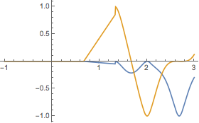
The onset of the conductor movements.

    ListPlot[{Table[{t, conductor??[t][[1]]}, {t, -1, 3, 0.01}],
      Table[{t, conductor??[t][[2]]}, {t, -1, 3, 0.01}]}, 
     PlotRange -> All, Joined -> True]

    With[{animationType = 2},
     scalefactors[1][t_] := 
      Switch[animationType, 1, {0.8, 1} , 2, loudness[t]];
     scalefactors[2][t_] := 
      Switch[animationType, 1, {1, 1} , 2, loudness[t]];
     scalefactors[3][t_] := 
      Switch[animationType, 1, {1, 1} , 2, loudness[t]];
     scalefactors[4][t_] := 
      Switch[animationType, 1, {1, 1} , 2, loudness[t]]
     ] 

christmasTreeWithSwingingOrnaments[t_, 
  conductorEnhancementFactor : fc_,  
  conductorCandleAngle : ?c_, topRotationAngle : ?_, 
  opts___] := 
 Graphics3D[{{Darker[Brown], stem}, 
   (* first voice *)
   branchOnStemWithBall[allBranches[[#]],
      scalefactors[1][t] voice??[1][t], 
      Darker[Yellow, -0.1],
      If[t < 0, {0, 0}, pendulum??[#][t]]] & /@ 
    voiceBranches[[1]],
   (* second voice *)

   branchOnStemWithBall[allBranches[[#]], 
      scalefactors[2] [t] voice??[2][t], 
      Blend[{Red, Pink}], 
      If[t < 0, {0, 0}, pendulum??[#][t]]] & /@ 
    voiceBranches[[2]],
   (* third voice *)

   branchOnStemWithFiveStar[allBranches[[#]], 
      scalefactors[3][t] voice??[3][t], randomColor[#], 
      Pi/4, If[t < 0, {0, 0}, pendulum??[#][t]]] & /@ 
    voiceBranches[[3]], 
   (* fourth voice *)

   branchOnStemWithCandle[#, 
      scalefactors[4][t] voice??[4][t], 
      Directive[White, Glow[GrayLevel[0.3]], Specularity[Yellow, 20]],
       0] & /@ allBranches[[voiceBranches[[4]]]], 
   (* conductor *)

   branchOnStemWithCandle[
    allBranches[[conductorBranch]] {1, 1, 1 + fc}, 
    conductor??[t], 
    Directive[Red, Glow[GrayLevel[0.1]],  
     Specularity[Yellow, 20]], ?c],
   Rotate[top, ?, {0, 0, 1}]
   }, opts, ViewPoint -> {2.8, 1.79, 0.1}, 
  PlotRange -> {{-8, 8}, {-8, 8}, {-2, 15}},
  Background -> RGBColor[0.998, 1., 0.867] ]

Use a low view point as trees are normally larger than humans.

Show[christmasTreeWithSwingingOrnaments[70, 0.5,  0.8, 2], 
 PlotRange -> All, Boxed -> False]

Let It Snow!

Some snow is is a must-be for a classic (white) Christmas. So, let's build some 3D snowflakes and then them fall down. Rather than solving PDEs (http://psoup.math.wisc.edu/papers/h3l.pdf), we will just use cellular automata on hexagonal grids to generate some snowflake-like shapes with hexagonal symmetry.

Snowflake shapes (2D)

Let's borrow some code from Ed Pegg's demonstration Snowflake-Like Patterns. I just import the notebook and programmatically extract the relevant cells that define the variables hex and snowflake.

ReleaseHold /@ (MakeExpression[#[[1]], StandardForm] & /@ 
    Take[Cases[
      Import["http://demonstrations.wolfram.com/downloadauthornb.cgi?\
name=SnowflakeLikePatterns"], Cell[_, "Input", ___], ?], 2]);

makeSnowflake[rule_, steps_] := 
 Polygon[hex[#] & /@ Select[Position[Reverse[CellularAutomaton[
       {snowflakes[[
         rule]], {2, {{0, 2, 2}, {2, 1, 2}, {2, 2, 0}}}, {1, 
         1}}, {{{1}}, 
        0}, {{{steps}}, {-steps, steps}, {-steps, steps}}]], 
     0], -steps - 1 < -#[[1]] + #[[2]] < steps + 1 &]] 

SeedRandom[33];
Table[Graphics[{Darker[Blue], 
   makeSnowflake[RandomInteger[{1, 3888}], 
    RandomInteger[{10, 60}]]}], {4}]

As some of snowflakes are disconnected, I select the ones that are interesting. I am also only are interested in snowflakes that are sufficiently complex.

denseFlakeQ[mr_MeshRegion] :=

 With[{c = RegionCentroid[mr], pts = MeshCoordinates[mr]},
           ( Divide @@ MinMax[EuclideanDistance[c, #] & /@ pts]) < 1/3]

randomSnowflakes[] := 
 Module[{sf},
  While[(sf = Module[{},
       TimeConstrained[
        hexagons = 
         makeSnowflake[RandomInteger[{1, 3888}], 
          RandomInteger[{10, 60}]];
        (Select[ConnectedMeshComponents[DiscretizeRegion[hexagons]], 
            (Area[#] > 120 && Perimeter[#]/Area[#] < 2 && 
               denseFlakeQ[#]) &] /.
           \
_ConnectedMeshComponents :> {}) // Quiet, 20, {}]]) === {}]; sf]

randomSnowflakes[n_] :=  
 Take[NestWhile[Join[#, randomSnowflakes[]] &, {}, Length[#] < n &], n]

SeedRandom[22];
randomSnowflakes[4]

normalizeFlake[mr_MeshRegion] := 
 Module[{coords, center, coords1, size, coords2},
  coords = MeshCoordinates[mr];
  center = Mean[coords];
  coords1 = (# - center) & /@ coords;
  size = Max[Norm /@ coords1];
  coords2 = coords1/size;
  GraphicsComplex[coords2, {EdgeForm[], MeshCells[mr, 2]}]]

Here are five flakes for further use.

3D Snowflake shapes

I extrude the 2D snowflakes to get 3D snowflakes.

make3DFlake[flake2D_] := 
 Module[{grc, reg, boundary, h, bc, rb, polys, pts},
       grc = flake2D[[1]];
       reg = MeshRegion @@ (grc /. _EdgeForm :> Nothing);

  boundary = (MeshPrimitives[#, 1] &@RegionBoundary[reg])[[All, 1]];
            h = RandomReal[{0.05, 0.15}];
       bc = 
   Join[#1, Reverse[#2]] & @@@ 
    Transpose[{Map[Append[#, 0] &, boundary, {-2}], 
      Map[Append[#, h] &, boundary, {-2}]}];
      rb = RegionBoundary[reg];
      boundary = (MeshCells[#, 1] &@rb)[[All, 1]];
      polys = 
   Polygon[Join[#1, Reverse[#2]] & @@@ 
     Transpose[{boundary, boundary + Max[boundary]}]];
      pts = 
   Join[Append[#, 0] & /@ MeshCoordinates[rb], 
    Append[#, h] & /@ MeshCoordinates[rb]];
  {GraphicsComplex[Developer`ToPackedArray[pts], polys],
   MapAt[Developer`ToPackedArray[Append[#, 0]] & /@ # &, flake2D[[1]],
     1],
   MapAt[Developer`ToPackedArray[Append[#, h]] & /@ # &, flake2D[[1]],
     1]}
  ]

listOfSnowflakes3D = make3DFlake /@ listOfSnowflakes;

Graphics3D[{EdgeForm[], #}, Boxed -> False, 
   Method -> {"ShrinkWrap" -> True}, ImageSize -> 120, 
   Lighting -> {{"Ambient", Hue[.58, .5, 1]}, {"Directional", 
      GrayLevel[.3], ImageScaled[{1, 1, 0}]}}] & /@ listOfSnowflakes3D

Model of a falling sheet

A simple 2D model of falling sheets was given by Tanabe and Kaneko in 1994. So, to get some intuition about possible fall shapes, we implement the model as an interactive demonstration.

Manipulate[ 
 Module[{eqs, nds, tmax, g = 10, ?, sign, V, x, y, u, 
   v, ?, ?, kpar = kperp/f, ? = 10^?exp},
  ? = ArcTan[u[t], v[t]];
  sign = Piecewise[{{1, (v[t] < 0 && 
         0 <= ? + ?[t] <= Pi) || (v[t] > 
          0 && -Pi <= ? + ?[t] <= 0)}}, -1];
  V = Sqrt[u[t]^2 + v[t]^2];
  eqs =
   {D[x[t], t] == u[t],
     D[y[t], t] == v[t],
     D[u[t], 
       t] == -(kperp Sin[?[t]]^2 + kpar Cos[?[t]]^2) u[
         t] +
                               (kperp - kpar) Sin[?[
          t]] Cos[?[t]] v[t] -

       sign Pi ? V^2 Cos[? + ?[t]] Cos[?],
     D[v[t], 
       t] == -(kperp Cos[?[t]]^2 + kpar Sin[?[t]]^2) v[
         t] +
                               (kperp - kpar) Sin[?[
          t]] Cos[?[t]] u[t] +

       sign Pi ?  V^2 Cos[? + ?[
           t]] Sin[?] - g,
     D[?[t], 
       t] == -kperp ?[
         t] - (3 Pi ? V^2/l) Cos[? + ?[
           t]] Sin[? + ?[t]],
     D[?[t], t] == ?[t]} /. kpar -> kperp/f; 
  nds = NDSolve[
     Join[eqs, {x[0] == 0, y[0] == 0, u[0] == 0, 
       v[0] == 0.01, ?[0] == 0, ?[0] == ?0}],
                            {x, y, u, v, ?, ?}, {t, 0, 
      T}, MaxSteps -> 2000] // Quiet; 
  tmax = nds[[1, 2, 2, 1, 1, 2]]; 
  Graphics[{Thickness[0.002], Gray,

    Table[Evaluate[
      Line[{{x[t], y[t]} - l/2 {Cos[?[t]], Sin[?[t]]},
                                                                {x[t],
            y[t]} + l/2 {Cos[?[t]], Sin[?[t]]}}] /. 
       nds[[1]]],
                                       {t, 0, tmax, tmax/n}],
                       Blue, 
    Line[Table[
      Evaluate[{x[t], y[t]} /. nds[[1]]], {t, 0, tmax, tmax/200}]]},
                        AspectRatio -> ar, Frame -> True, 
   PlotRange -> All]],
 "system parameters",
 {{kperp, 5.1, Subscript["k", "?"]}, 0.01, 10, 
  Appearance -> "Labeled"},
 {{f, 145, 
   Row[{Subscript["k", "?"], "/", 
     Subscript["k", "?"]}]}, 0.01, 200, 
  Appearance -> "Labeled"},
 {{?exp, -0.45, Log["?"]}, -3, 1, Appearance -> "Labeled"},
 {{l, 0.63}, 0.01, 10, Appearance -> "Labeled"} ,
 Delimiter,
 "fall parameters",
 {{?0, 1, Subscript["?", "0"]}, -Pi, Pi, 
  Appearance -> "Labeled"},
 {{T, 2, "falling time"}, 0, 10, Appearance -> "Labeled"} ,
 Delimiter,
 "plot",
 {{ar, 1, "aspect ratio"}, {1, Automatic}},
 {{n, 200, "snapshots"}, 2, 500, 1}]

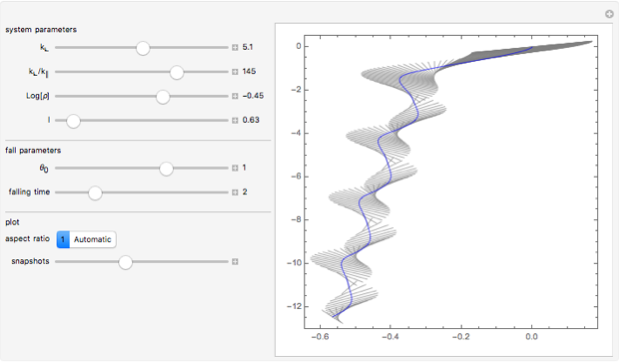
I will model the falling process phenomenologically and heuristically rather than through the differential equation solution. With the density values of snowflakes and air, together with their thickness/area ratio they fall mostly straight down, with some small lateral movements and internal rotations.

Falling Snowflakes

Model internal rotations about the center of mass as well as some small lateral movements.

randomParametrizedRotationMatrix[n_, ?_] := Function @@ {?,
    Module[{phi, s, c},

     Do[phi[i] =  
       Sum[RandomReal[{-1, 1}] Sin[
          RandomReal[{0, n}] ? + 2 Pi RandomReal[]], {n}];
               {c[i], s[i]} = {Cos[phi[i]], Sin[phi[i]]}, {i, 3}];
            {{c[1], s[1], 0}, {-s[1], c[1], 0}, {0, 0, 1}}.
             {{c[2], 0, s[2]}, {0, 1, 0}, {-s[2], 0, c[2]}}.
             {{1, 0, 0}, {0, c[3], s[3]}, {0, -s[3], c[3]}}]};

randomParametrizedPathFunction := Function[t,
  Evaluate[{RandomReal[{-5, 5}] + 
     Sum[RandomReal[{-1, 1}]/# Cos[2 Pi # t] &[
       RandomReal[{1, 4}]], {k, 5}], 

    RandomReal[{-5, 5}] + 
     Sum[RandomReal[{-1, 1}]/# Cos[2 Pi # t] &[
       RandomReal[{1, 4}]], {k, 5}], 
                      RandomReal[{2, 12}] - RandomReal[{1.5, 2.5}] t}]]

SeedRandom[55];
Do[rotMat[j] = randomParametrizedRotationMatrix[3, ?];
      trans[j] = randomParametrizedPathFunction;
      snowflakeColor[
   j] = {{"Ambient", 
    Hue[RandomReal[{0.55, 0.6}], RandomReal[{0.48, 0.52}], 
     RandomReal[{0.95, 1}]]}, {"Directional", 
    GrayLevel[RandomReal[{0.28, 0.32}]], 
    ImageScaled[{1, 1, 0}]}}, {j, Length[listOfSnowflakes]}]

fallingSnowflake[flake_, {t_, ?_}] := 
 flake /. GraphicsComplex[cs_, rest__] :> 
   GraphicsComplex[(?.# + t) & /@ cs, rest]

Manipulate[
 Graphics3D[{EdgeForm[],
   Table[{Lighting -> snowflakeColor[k], 
     fallingSnowflake[
      listOfSnowflakes3D[[k]], {trans[k][t], rotMat[k][t]}]}, {k, 
     Length[listOfSnowflakes3D]}] },
  PlotRange -> 6, ViewPoint -> {0, -10, 0}, ImageSize -> 400],
 {{t, 3.2}, -5, 20}]

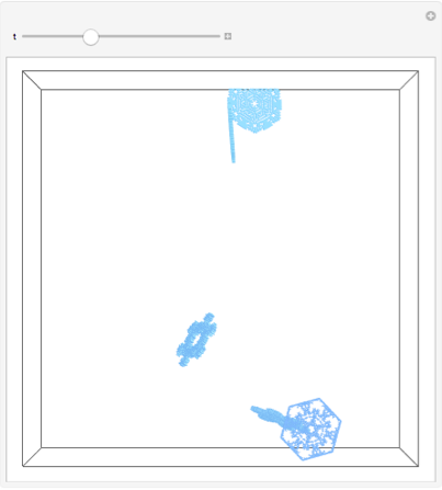
For the full animation a few hundred snowflakes were used.

Making the Animation Frames

Now start the animation by extending the conductor branch and also rotate the top while the music is playing. Then, we will listen and view one verse. Then, we will move once around the tree and have some snowfall. And then comes the wild part where the tree swings its ornaments ecstatically around before calming down and retracts its conductor branch. I generate 24 frames for each second of sound.

conductorBranchMaxfactor = 0.5;
conductorBranchLength[t_] := 
  conductorBranchMaxfactor*
   Which[t < -3, 0, -3 < t <= 0, (t + 3)/3., 0 <= t <= tMax, 1, 
    tMax < t < tMax + 3, (1 - (t - tMax)/3), True, 0];

topRotation[t_] := 
  Which[t < -3 || t > tMax + 3, 0, 
   True, (1. - Cos[(t + 3)/(tMax + 6)]) 20 2 Pi];

viewPoint[t_] := 
 With[{vp = {2.8, 1.79, 0.1}},
  Which[t < changeTimeList[[1]] || t > changeTimeList[[2]], vp,
              changeTimeList[[1]] <= t <= changeTimeList[[2]],
              Module[{t0 = changeTimeList[[1]], 
                             ?t = 
      changeTimeList[[2]] - changeTimeList[[1]], ?vp},
               ?vp = -Pi (1 - 
        Cos[ Pi (t - t0)/?t]); {{Cos[?vp], 
        Sin[?vp], 0}, {-Sin[?vp], Cos[?vp], 
        0}, {0, 0, 1}}.vp +
         {0, 0, 2 Sin[Pi (t - t0)/?t]^4 }]]] 

ParametricPlot3D[
 viewPoint[t], {t, changeTimeList[[1]], changeTimeList[[2]]}, 
 BoxRatios -> {1, 1, 1}]

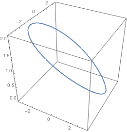
animationFrame[t_] := 
 Show[christmasTreeWithSwingingOrnaments[t, conductorBranchLength[t], 
   1.4 conductorBranchLength[t], topRotation[t]],
  Background -> None, Boxed -> False, SphericalRegion -> True, 
  ViewPoint -> viewPoint[t]]

A last test before running the export of the frames that will take a few hours:

    animationFrame[35]

framesPerSecond = 24;
animationFrameDirectory = 
  "/Users/mtrott/Desktop/ConductingChristmasTreeAnimationFrames/";

Monitor[
 Do[
  With[{t = -3 + 1/framesPerSecond (frame - 1)}, gr = animationFrame[t];
   Export[animationFrameDirectory <> IntegerString[frame, 10, 4] <> ".png", gr,
                  ImageSize -> 1800, Background -> None] 
   ],
  {frame, 1, framesPerSecond (100 + 2 3)}],
 Row[{frame, " | ", Round[MemoryInUse[]/1024^2], "\[ThinSpace]MB" }]
 ]

Now use your favorite film editing software (like Adobe After Effects) and put the moving tree, the sound, and the snowfall together.