Here is for example the magnetic scalar field:

(* Get the "magnetic scalar potential" *)

rbm = Entity["PhysicalSystem", "RectangularBarMagnet"][
   "MagneticScalarPotential"];

(* Make "magnetic scalar potential" Active and replace the \ subscripted parameter with a non-subscripted one *)

rbmmsp[m0_, a_, b_, c_, x_, y_, z_] := 
  Activate[rbm] //. 
   QuantityVariable[Subscript["M", 0], "Magnetization"] -> 
    QuantityVariable["m0", "Magnetization"];

(* Create the magnetic field *)

rbmmf[m0_, a_, b_, c_, x_, y_, 
   z_] := -D[
    rbmmsp[m0, a, b, c, x, y, 
     z], {{QuantityVariable["x", "Length"], 
      QuantityVariable["y", "Length"], 
      QuantityVariable["z", "Length"]}}];

(* Create the non-QuantityVariable /nqv/ magnetic field *)

nqvrbmmf[m0_, a_, b_, c_, x_, y_, z_ ] := 
 rbmmf[m0, a, b, c, x, y, 
   z] /. {QuantityVariable["m0", "Magnetization"] -> m0, 
   QuantityVariable["x", "Length"] -> x, 
   QuantityVariable["y", "Length"] -> y, 
   QuantityVariable["z", "Length"] -> z, 
   QuantityVariable["a", "Length"] -> a , 
   QuantityVariable["b", "Length"] -> b, 
   QuantityVariable["c", "Length"] -> c} 

Now the field can be displayed for example by ContourPlot3D as:

ContourPlot3D[
Evaluate[Norm[nqvrbmmf[mu0, a, b, c, x, y, z]]], {x, -1.5*a, 
5.5*a + 4*gap}, {y, -2*b, 2*b}, {z, -3.5*c, 1.5*c}, 
MaxRecursion -> 0, PlotPoints -> 30, 
Contours -> {10^2, 5*10^2, 10^3, 5*10^3, 10^4, 5*10^4, 10^5, 
2*10^5}, Mesh -> None, 
ContourStyle -> (Directive[Opacity[0.66], #1] &) /@ 
Table[ColorData["RedBlueTones"][xi], {xi, 1, 0, -1/16}], 
BoxRatios -> Automatic]// ReplaceAll[#, {mu0 -> 10^6, a -> 0.01, b -> 0.01, c -> 0.01, gap -> 0.001}] & // Quiet

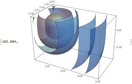
or with VectorPlot3D:

VectorPlot3D[
    nqvrbmmf[mu0, a, b, c, x, y, z] , {x, -1.5*a, 
     5.5*a + 4*gap}, {y, -2*b, 2*b}, {z, -3.5*c, 1.5*c + R}, 
    VectorPoints -> {40, 20, 30}, BoxRatios -> Automatic, 
    Axes -> True, PlotLegends -> Automatic, 
    PlotRange -> {{-0.015, 0.059}, {-0.02, 0.02}, {-0.035, 0.115}}] //
    ReplaceAll[#, {mu0 -> 10^6, a -> 0.01, b -> 0.01, c -> 0.01, 
      gap -> 0.001, R -> 0.1}] & // Quiet 

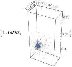
Now, I can "move" this field for example by the z-axis up by replacing the "z" variable with "z-R" variable in the field signature and display with VectorPlot3D like this:

VectorPlot3D[
   nqvrbmmf[mu0, a, b, c, x, y, z - R] , {x, -1.5*a, 
    5.5*a + 4.0*gap}, {y, -2.0*b, 2.0*b}, {z, -3.5*c, 1.5*c + R}, 
   VectorPoints -> {40, 20, 30}, BoxRatios -> Automatic, Axes -> True,
    PlotLegends -> Automatic, 
   PlotRange -> {{-0.015, 0.059}, {-0.02, 0.02}, {-0.035, 0.115}}] // 
  ReplaceAll[#, {mu0 -> 10^6, a -> 0.01, b -> 0.01, c -> 0.01, 
     gap -> 0.001, R -> 0.1}] & // Quiet

My problem is that in further calculations then I always have to refer to "z-R" instead of just simple a "w". I would like to do something like this:

tnqvrbmmf = 
 TransformedField["Cartesian" -> "Cartesian", 
   nqvrbmmf[mu0, a, b, c, x, y, z], {x, y, z - R} -> {u, v, ww}] // 
  Simplify

But it is complaining that {x,y,-0.1+z} is not a non-empty list of valid variables and after some time crashing Mathematica death on.