Consistency in foreign exchange derivatives is being discussed in the below note where we look at the problem from the probability measure perspective. We review option valuation from both sides of the FX contract and conclude that investors' preferences are subject to different probability measures when the FX rate inverts. Following this we prove the validity of Siegel's paradox.

Introduction

Foreign exchange options are the oldest options in the market with a long history of trading. As such, they have been deeply-researched and are well-understood. Nevertheless, we return to this topic to look at the product consistency, since this may still not be entirely clear. We review this consistency from both - domestic and foreign perspectives and show what adjustments are required to ensure the options are arbitrage-free when the investor's position changes

Foreign exchange options - 1st currency measure

Foreign e change options are financial contracts on FX rate -i.e. rate of exchange of currency 1 fro currency 2. GBP/USD or EUR/USD are examples of such currency pairs. Options are essentially contracts on the future spot FX rate. We will demonstrate the exposition to this subject using EUR/USD exchange rate. This is the rate that sets the exchange equation of $X = [Euro]1

A reader familiar with the equity derivatives market will immediately spot the similarity between these two products. If the equity growth rate under the risk-neutral measure is the risk-free rate r, the equity pays a continuous dividend yield q and the price process is assumed log-normal, this is identical to the FX when we express r and the USD risk-free rate and q as the equivalent EUR risk-free rate.

Looking at his from the USD-perspective, we can express the EUR/USD FX process as:

$$dF = F (r-q) dt + ? F dW$$

This is a well-known log-normal process for the exchange rate where F represents the EUR/USD rate, [Sigma] is the FX rate volatility and W represents a Wiener process under the USD-measure.

Pricing option on this future rate is trivial - this is an option buy [Euro] 1 for K USD and time T. Therefore from the USD-perspective, the option pays: Max[0,F-K] where K is the strike exchange rate. Pricing this option in Mathematica is easy - we build the standard Ito Process for initial value F0.

ipUSD = Refine[
ItoProcess[{(r - q)*F, \[Sigma]*F}, {F, F0}, t], {\[Sigma] > 0, 
F[t] > 0, t > 0}];
{Mean[ipUSD[t]], Variance[ipUSD[t]]}

{E^((-q + r) t) F0, E^(-2 q t + 2 r t) (-1 + E^(t $[Sigma]^2)) F0^2}

The option premium from the USD-perspective is an expectation of the above Ito Process.

usdOpt = Exp[-r*t]*
Expectation[Max[F[t] - K, 0], F \[Distributed] ipUSD, 
Assumptions -> 
F0 > 0 && K > 0 && \[Sigma] > 0 && t > 0 && r > 0 && q > 0] // 
Simplify

-(1/2) E^(-r t) (-2 E^((-q + r) t) F0 + 
E^((-q + r) t)
F0 Erfc[(t (-2 q + 2 r + \[Sigma]^2) + 2 Log[F0] - 2 Log[K])/(
2 Sqrt[2] Sqrt[t] \[Sigma])] + 
K Erfc[(t (2 q - 2 r + \[Sigma]^2) - 2 Log[F0] + 2 Log[K])/(
2 Sqrt[2] Sqrt[t] \[Sigma])])

Foreign exchange options - 2nd currency measure

Now we touch upon a part that is less clear - what if the option buyer (seller) thinks from the the EUR-perspective? This is quite legitimate as option buyers or sellers can have different preferences when entering into the option contract. How do we ensure that the option contract is consistent from each side-perspective?

Let's spell out the EUR investor position by replicating the USD investor side

• EUR riskless process is dP = P q dt and not dB = B r dt representing USD process
• The exchange-rate is now 1/F and not F

• When SDE for the exchange rate from the USD-point of view is the one above, then for the process 1/F this becomes - using Ito lemma:

  f = 1/F;
  ip02 = Refine[
  ItoProcess[{(r - q)*F, \[Sigma]*F, f}, {F, F0}, t], {\[Sigma] > 0, 
  F[t] > 0, t > 0, r > 0, q > 0}];
  ipEUR = ItoProcess[ip02] // Simplify     
  
  ItoProcess[{{(-q + r) F[t], (q - r + \[Sigma]^2)/
  F[t]}, {{\[Sigma] F[t]}, {-(\[Sigma]/F[t])}}, \[FormalX]1[
  t]}, {{F, \[FormalX]1}, {F0, 1/F0}}, {t, 0}]
  

The inverted FX rate (USD/EUR) produces different Ito Process than the one observed on the USD-side. This is clear from the definition below:

$$d(1/F) = (1/F) (q-r+?^2) dt -? (1/F) d W$$

Our objective is to find probability measure under which the FX option priced in the first section from the USD-perspective will be identical to the one priced from the EUR-perspective. Let's take all tradable components of the trade: (i) USD risk-free discount factor B , (ii) FX rate EUR/USD F and (iii) EUR discount factor P. Based on this we define:

• USD-risk-free process converted to EUR: B/F

• Discounted value of the above : B/ (F P)
  So, we need a multi-dimensional Ito process to model B/(F P)

  ip03 = Refine[
      ItoProcess[{{0, r B, q P}, {F \[Sigma], 0, 0}, 
        B/(P F)}, {{F, B, P}, {F0, B0, P0}}, t], {\[Sigma] > 0, r > 0, 
       q > 0, t > 0}] // Simplify;
  ipEUR2 = ItoProcess[ip03]
  
  ItoProcess[{{0, r B[t], q P[t], (-q B[t] + r B[t] + \[Sigma]^2 B[t])/(
     F[t] P[t])}, {{\[Sigma] F[t]}, {0}, {0}, {-((\[Sigma] B[t])/(
       F[t] P[t]))}}, \[FormalX]1[t]}, {{F, B, P, \[FormalX]1}, {F0, B0,
      P0, B0/(F0 P0)}}, {t, 0}]
  

From the above Ito Formula, we extract two coefficients - drift and volatility of B/(F P) and create new ItoProcess that reflects the changes when FX inversion occurs.

Flatten[ipEUR2[[1]]];
dr = %[[4]] /. {F[t] -> 1, B[t] -> 1, P[t] -> 1}
vl = %%[[8]] /. {F[t] -> 1, B[t] -> 1, P[t] -> 1}
ItoProcess[{dr F, vl F}, {F, F0}, t];
ipEUR3 = ItoProcess[%]

-q + r + \[Sigma]^2
-Sigma
ItoProcess[{{(-q + r + \[Sigma]^2) F[t]}, {{-\[Sigma] F[t]}}, 
  F[t]}, {{F}, {F0}}, {t, 0}]  

It is quite clear that the inverted FX rate process USD/EUR is indeed different to the one observed in the EUR/USD case.

In order to prove this consistency, we need to show that FX call option on EUR/USD from EUR point of view is identical to the one priced from the USD-perspective. So, we need to prove that:

E^(-r t) Subscript[E, USD] ( Max[ Subscript[F, t]-K,0]) = E^(-q t) Subscript[F, 0]   Subscript[E, EUR] (  (1/Subscript[F, t])  Max[1/Subscript[F, t]-K,0] )

This is because the expectation of the option payoff has to be converted back into EUR. All we need to price this option is use the following expectation:

eurOpt = F0 Exp[-q t] Expectation[Max[F[t] - k, 0]/F[t], 
    F \[Distributed] ipEUR3, 
    Assumptions -> 
     F0 > 0 && k > 0 && \[Sigma] > 0 && t > 0 && r > 0 && q > 0] // 
  Simplify

1/2 E^(-(q + r) t) (E^(r t) F0 - E^(q t) k + 
   E^(r t) F0 Erf[(
     t (-2 q + 2 r + \[Sigma]^2) + 2 Log[F0] - 2 Log[k])/(
     2 Sqrt[2] Sqrt[t] \[Sigma])] + 
   E^(q t) k Erf[(t (2 q - 2 r + \[Sigma]^2) - 2 Log[F0] + 2 Log[k])/(
     2 Sqrt[2] Sqrt[t] \[Sigma])])

To finalise this exercise, we compute both option premiums:

usdNum = usdOpt /. {F0 -> 1.35, t -> 0.5, K -> 1.36, \[Sigma] -> 0.2, 
   r -> 0.01, q -> 0.012}
eurNum = eurOpt /. {F0 -> 1.35, t -> 0.5, k -> 1.36, \[Sigma] -> 0.2, 
   r -> 0.01, q -> 0.012}
usdNum - eurNum // Chop

0.070452

0.070452

0

Both option premium are the same. This proves they are consistent.

Siegel's paradox

In the context of the above discussion, it is worth mentioning Siegel's paradox as it directly links the FX processes to probability measures. Let's start again with the definition of FX evolution from the USD-perspective . Under the USD probability measure (USD risk-neutral process) we showed earlier that this was:

$$dF = F (r-q) dt + ? F dW$$

The expected future FX rate - the FX Forward at time t is an expectation of Subscript[F, t] under the USD measure:

usdExp = Expectation[F[t], F \[Distributed] ipUSD, 
Assumptions -> F0 > 0 && \[Sigma] > 0 && t > 0 && r > 0 && q > 0] //
Simplify 
E^((-q + r) t) F0

Let's look now at EUR-investor point of view. (S)he can do similar calculation and under her/his neutral measure the USD/EUR process follows:

$$d(1/F) = (1/F) (q-r) dt + (1/F) ? dW$$

So, the forward rate of 1/F (EUR per USD) is:

eurExp2 = 
Expectation[1/F[t], F \[Distributed] ipEUR3, 
Assumptions -> F0 > 0 && \[Sigma] > 0 && t > 0 && r > 0 && q > 0] //
Simplify 

E^((q - r) t)/F0

This seems logical, since inverted FX is simply :1/F. Here lies the problem: since 1/F is essentially a convex function, by Jensen's inequality:

(E[F])^-1 < E [F^-1]

when both expectations are taken w.r.t to same probability measure = i.e. calculated with the same distribution and F is non-constant. This runs contrary to our assertion above where we outlined the conditions for consistency - i.e. different probability measure.

Siegel's paradox is simply a statement confirming that the spot rate inversion does not extrapolate to the forward space and the forward FX rate in general cannot be an unbiased estimate of future spot FX rate. At least not simultaneously for both sides of the contract due to 'convexity' effect in the inverted FX function. This is due to the Jensen's inequality statement above. If the property holds for the USD-investor, it cannot be true for the EUR investor and vice-versa since their forward expectation are subject to different probability measures.

We prove this on the simple case - define standard Ito process and then take the expectations for for F and 1/F

ip05 = Refine[
ItoProcess[{(r - q)*F, \[Sigma]*F}, {F, F0}, t], {\[Sigma] > 0, 
F[t] > 0, t > 0, r > 0, q > 0}];
usdFwrd = 
Expectation[F[t], F \[Distributed] ip05, 
Assumptions -> F0 > 0 && \[Sigma] > 0 && t > 0 && r > 0 && q > 0] //
Simplify
eurFwrd = 
Expectation[1/F[t], F \[Distributed] ip05, 
Assumptions -> F0 > 0 && \[Sigma] > 0 && t > 0 && r > 0 && q > 0] //
Simplify

E^((-q + r) t) F0
E^(t (q - r + \[Sigma]^2))/F0

We see that the FX forwards are different as their are taken from different probabilities (with different mean and variance). The forward of 1/F depends also on volatility whereas F does not. Let's show the validity of Jensen's inequality: 1/ Subscript[F, USD] and Subscript[F, EUR]

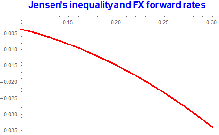
fxMeanDiff = 1/usdFwrd - eurFwrd // Simplify
-((E^((q - r) t) (-1 + E^(t \[Sigma]^2)))/F0)

Since the above quantity is negative, this shows that indeed

(E[Subscript[F, t]])^-1 < E[Subsuperscript[F, t, -1]]

Plot[fxMeanDiff /. {F0 -> 1.35, r -> 0.01, q -> 0.0045, 
   t -> 0.5}, {\[Sigma], 0.1, 0.3}, 
 PlotLabel -> 
  Style["Jensen's inequality and FX forward rates", {15, Bold}, Blue],
  PlotStyle -> {Thick, Red}]

Jensen's inequality effects increases with volatility. On the other hand, the only instance when both forwards will be consistent w.r.t the same probability occurs when [Sigma]=0. Since this is never the case, we conclude that Siegel's paradox holds.

Conclusion

The objective of this note was to present the FX derivatives - forwards and options from different perspective. Whilst the FX spot market is reasonably simple, derivatives are more complicated, especially when we start looking at them from each contractual perspective. Change of probability measure, and hence different probabilities are required to ensure consistency. Existence of Siegel's paradox proves this.

Change of probability measure is handled implicitly by Mathematica once the FX process is correctly defined. The same applies to proving of Siegel's paradox.

Attachments: