Click on the image to zoom. Then click your browser back button to return to reading the post.

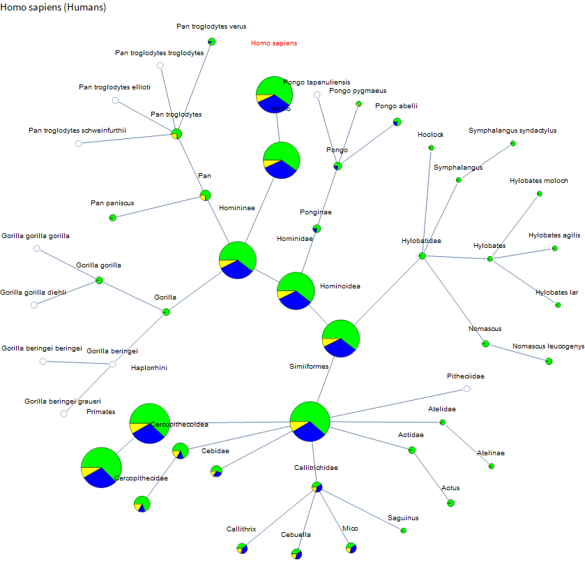
• Pie chart size is related to total sequence count
• Green is normal
• Blue is EST
• Yellow is GSS

See detailed explanations in the text below.

Often when I see an organism, I wonder if we've sequenced its genome. And if not, how much we've sequenced of related species. The NCBI Nucleotide web interface (although calling it "GenBank" still seems easier) has a lot of technical features to help professional biologists who are already well versed in their specialization area, but I wanted to see a graph plot showing related taxa to a target species and how much data is available for each. This way, if I'm interested in an organism that isn't well studied I can quickly find the most similar thing with available data. I started this last night and I'm already finding it interesting, so I figured I'd share.

Downloading all of GenBank for this isn't practical, so we'll just have a taxonomy in memory and send queries to the website for the specific taxa we want sequence counts for. Now you could get started by downloading some of Wolfram's species data (a very simple line of code), but that mechanism seems currently suited for smaller amounts of data, so I just downloaded a snapshot of the data from ITIS. It's less complete than the Wolfram data which uses a combination of databases like the Catalogue of Life, which includes ITIS. But ITIS alone doesn't require ordering DVDs and is still very thorough by most people's standards.

I made a simple CSV from the ITIS data and attached it at the end. So I import that and use the parent links to make a graph.

taxa = Import["taxa.csv"] // 
   Function[rows, 
    Map[AssociationThread[First@rows -> #] &, Rest@rows]];

tsnToName = #tsn -> #@"complete_name" & /@ taxa // Association;

taxonomy = 
  tsnToName[#tsn] <-> tsnToName[#@"parent_tsn"] & /@ taxa // Graph;

So taxonomy is our main hierarchy from which we will take local subgraphs around our target species. The NCBI does offer a reasonably sized download that will help reduce the amount of requests we send to their servers. We can download a list of all of the species which have at least one published sequence from their taxonomy section, so we don't have to waste time or server resources on queries that return nothing. Specifically we want the names.dmp file from this ZIP in their FTP section. So I'll import that and make a quick lookup table to check if any sequences are available for a given name.

names = Import["names.dmp", "Text"] // StringDrop[#, -2] & // 
     StringSplit[#, "\t|\n"] & // StringSplit[#, "\t|\t"] & // 
   Map[AssociationThread[{"id", "name", "unique", "class"} -> #] &];

sequencesExist = 
  AssociationMap[True &, 
   Select[names, #class == "scientific name" &][[All, "name"]]];

We have one more boring data import section to get out of the way. The NCBI apparently has quite a thorough API. It even has an introductory video. The first set of numbers I wanted though are right at the top of the search results page, so I just used scraping for now to hit my sub 24 hour goal. This code is rough and I will replace it with proper API calls as I move forward with the project. Basically you just do a search like "scientific name"[Organism] to limit to just the results we want. Then I pull out the total sequence count, and the EST and GSS count. Most nucleotide sequence data is not as well curated as a whole, annotated genome. ESTs and GSSs are short snippets of data that are captured while a gene is being expressed or have not been assembled into a larger sequence yet.

parseNucleotides[text_] := 
 StringCases[text, 
   Shortest["Found " ~~ a : DigitCharacter .. ~~ " " ~~ __ ~~ "\n"] :>
     ToExpression@a] // If[Length@# > 0, First@#, 1] &

parseEST[text_] := 
 StringCases[text, 
   Shortest["EST ( " ~~ a : DigitCharacter .. ~~ " " ~~ __ ~~ "\n"] :>
     ToExpression@a] // If[Length@# > 0, First@#, 0] &

parseGSS[text_] := 
 StringCases[text, 
   Shortest["GSS ( " ~~ a : DigitCharacter .. ~~ " " ~~ __ ~~ "\n"] :>
     ToExpression@a] // If[Length@# > 0, First@#, 0] &

sequenceCount[name_] := 
 sequenceCount[name] = 
  Import["https://www.ncbi.nlm.nih.gov/nuccore/?term=%22" <> 
     URLEncode@name <> "%22%5BOrganism%5D"] // {parseNucleotides@#, 
     parseEST@#, parseGSS@#} &

OK, so let's choose a species and extract a subgraph! Let's start with us! Homo sapiens. I just take the neighborhood graph of a certain size and then filter out any dangling leaves that don't have any sequence data (although that is optional if you want). I start with a small neighborhood size and then gradually increase it until I get a vertex count around 50. For humans that was 7, but for a Bermuda grass size 3 already gives you 400 vertices.

species = "Homo sapiens";

graph = NeighborhoodGraph[taxonomy, species, 7] // 
   Subgraph[#, 
     Select[VertexList@#, 
      Function[name, 
       sequencesExist@name || VertexDegree[#, name] > 1]]] &;
VertexCount@graph

Now let's download the sequence counts for all of our vertices. Depending on how many you have it could take several minutes, so let's throw a progress bar on it.

i = 0;
Monitor[counts = (i++; sequenceCount@#) & /@ VertexList@graph, 
  ProgressIndicator[i, {0, Length@VertexList@graph}]];

Now we just visualize the results. I do one more pass of pruning to exactly 50 nodes. I sort vertices first by distance from the target and then by decreasing number of sequences. This is just to keep the graphs interesting and reasonably sized. Even with that, they will tend to be very wide graphs, so I went with a radial layout instead of a layered layout. For the vertices, I just used a pie chart (size is related to total sequence count, green is normal, blue is EST, and yellow is GSS). For ones that just had one sequence the search page takes you to the sequence not the search results page, so I just show a small gray circle because I haven't parsed anything interesting from those pages yet. Each vertex has a tooltip with the exact counts and is a hyperlink to help with looking up scientific names. Target species name is in red.

df = FindShortestPath[graph, All, All];

Graph[Subgraph[graph, 
  Take[SortBy[
    VertexList[
     graph], {Length@df[species, #] &, -sequenceCount[#][[1]] &}], 
   UpTo@50]],
 VertexSize -> 
  Thread[VertexList@
     graph -> .7*3 Rescale[N@Sqrt[counts[[All, 1]]]] + .3],
 VertexShapeFunction -> Function[{pos, name, size},
   Hyperlink[
    If[sequenceCount[name][[1]] > 1,
     Tooltip[
      Inset[PieChart[
        sequenceCount[
          name] // {#[[1]] - (#[[2]] + #[[3]]), #[[2]], #[[3]]} &, 
        ChartStyle -> {Green, Blue, Yellow}, 
        LabelingFunction -> None], pos, {0, 0}, size], 
      Column@{name, Row@{"Total: ", sequenceCount[name][[1]]}, 
        Row@{"EST: ", sequenceCount[name][[2]]}, 
        Row@{"GSS: ", sequenceCount[name][[3]]}}],
     Circle[pos, size[[1]]/2]
     ],
    "https://www.google.com/search?q=" <> URLEncode[name]]],
 VertexLabels -> Placed[Automatic, Above],
 VertexLabelStyle -> {species -> Red},
 GraphLayout -> "RadialDrawing"]

And that's it! Let's look at some results.

As you follow the trail of increasing circles you are moving up the taxonomy, although this one is dominated by the amount of data on humans. I find it interesting though that we have almost as much data on marmosets, etc as we do on chimpanzees (although a larger portion is just ESTs).

The impetus for this project was actually me researching the genetics of lawn grasses. Here are the results for Bermuda grass.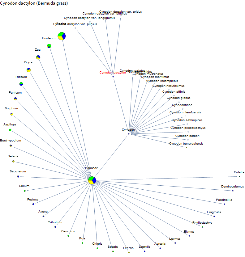

I knew that corn and rice are relatively well studied. But I didn't know about the little burst of data around African Bermuda grass or that barley has even more data than corn. So the project is already a success! Let's check out dogs.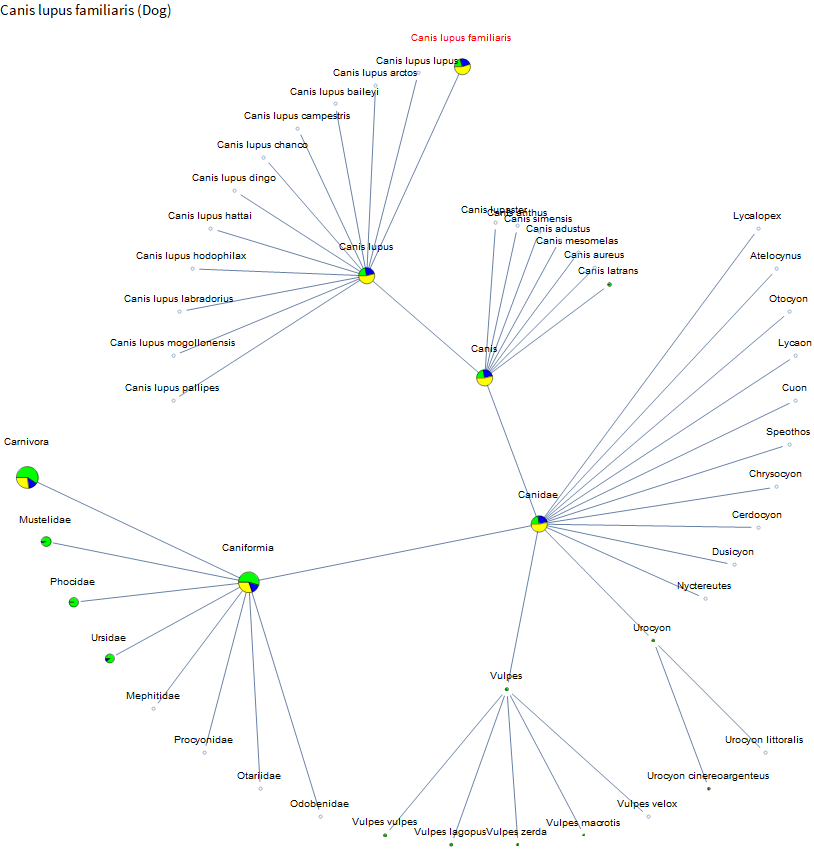

There is a fair amount of data on dogs, but there is very little on their relatives. A bit on coyotes and foxes. But we have much more data on the family containing weasels than on coyotes and foxes. Perhaps because there are more pets in the mustelids, and it's a large family. I've spent the past few weeks on vacation in Hawaii and French Polynesia. There were a lot of peacocks running around the ranch at our Airbnb in Hawaii. Let's check them out.

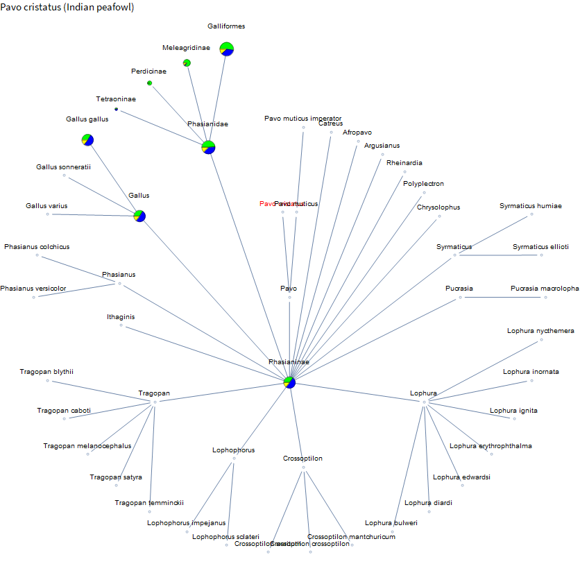
Not much data until you get over to chickens. French Polynesia is known for clear water and beautiful reefs. And you might see some blacktip reef sharks. I didn't see any this trip, but I have seen them in the Maldives, so let's take a look.

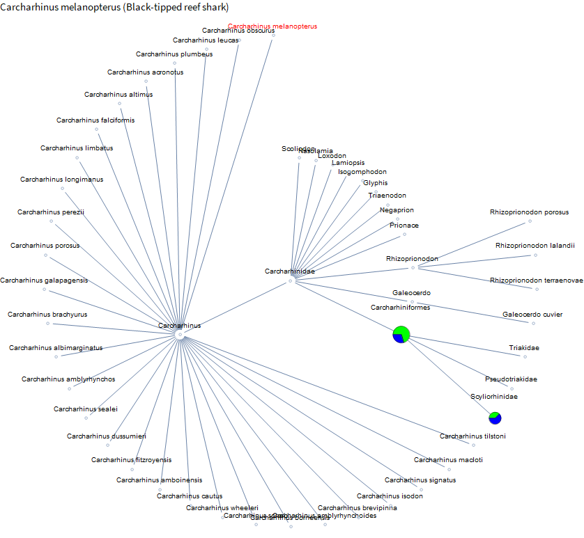
Not much available on specific sharks yet except for catsharks. Perhaps again because they are often kept by people in aquaria.

If you want to explore, the notebook and one of the data files you need is attached. The other data file you need is linked in the text above.

Attachments: