Hello Arm,

There are many ways to accomplish what you're trying to do, and Manipulate certainly isn't the only option. For the sake of my answer, I've chosen to use Manipulate since that's what you were attempting in your question, but it's worth mentioning that Manipulate isn't always the ideal solution. In my opinion, Manipulate is best used when you don't know in advance what sets of parameters you will want and you would like to tinker with them before making a decision. On the other hand, if you know that you will want graphs with specific sets of parameters, then it might be more efficient to use a function like Table or Map, depending on how you've set up your problem.

For example, if you have a simple equation of a line, and want to see what it looks like when the slope varies between 0 and 2 in steps of 0.5 (m= 0, m=0.5 ... m=2), then you could try this instead:

Show[Table[Plot[m x +2,{x,-5,5}],{m,0,2,0.5}]]

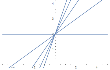
In this case Table is much faster to use than Manipulate because we know what values for the slope we want ahead of time. With a bit more work, we could still customize the colors, add labels, or whatever else we wanted.

Before I get into the solution that I came up with, I want to mention a few other tips that you might find helpful for the future. First, if you didn't know, you can actually give multiple equations to the Plot function in the form of a list instead of using Plot on each one separately and combining them with Show. For example:

Plot[{Sin[x],Cos[x+1.6], Sin[x]/x},{x,-5,5}, PlotLabels-> "Expressions"]

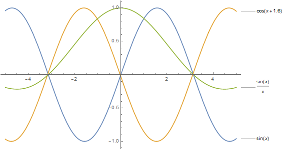
As you can see, this has the added benefit of automatically giving each curve a unique color, and allows you to easily identify them all with options like PlotLabels or PlotLegends. A more complete discussion of how you can use Plot is probably outside the scope of this question, but it's worth digging into the documentation a bit more if you're going to be doing a lot of plotting in the near future.

Another point I wanted to mention was that when you attempted to use H1, H2 and H3 in Manipulate in your example, you never actually gave the functions the information they needed to draw the plots. For example, in your definition of H1:

H1[x_, y_, b_, c_] := Plot[ Sin[x/b] + Cos [12 c], {x, -100, 100} , PlotStyle -> Green , PlotRange -> Automatic];

You used a delayed definition, so Mathematica holds that code in a symbolic form until it's given the information it needs to actually evaluate it. Using the definition above, we still need to supply values for the arguments in order to get a result, like this:

H1[1,2,3,4]

Unfortunately, with the definition of H1 as you wrote it, trying to evaluate H1 will result in an error message. That's because you included x as both an argument to the function and as the iterator for the Plot function. When Mathematica evaluates this, it replaces all instances of x, y, b and c in your definition of H1 with the arguments you supply. In this case, if we try to use the function as I did above, what you end up with looks like this:

Plot[ Sin[1/3] + Cos [48], {1, -100, 100} , PlotStyle -> Green , PlotRange -> Automatic]

This is not valid syntax, so it's returned in symbolic form and an error message is generated. It's also worth noting that you added the argument y to H1, but it's not actually used anywhere in the function's definition. Taking all of this into account, it would be better to rewrite H1, and then use it like this:

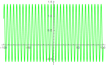
H1[b_,c_]:=Plot[Sin[x/b]+Cos[12 c],{x,-100,100}, PlotStyle-> Green];
H1[1,2]

Note that in the above example, I omitted your use of PlotRange because you used Automatic. It wasn't really necessary since Automatic is the default value. I hope that this is helpful to you, and I apologize if I've repeated things you already knew. It's difficult to guess what people do or don't know already, and I like to err on the side of caution.

So, now to the actual question you asked! The short answer is that yes, there is a way to do what you wanted with Manipulate. In my code, I chose to include a button that progressively adds functions to a list to be plotted when you press it. That is, it takes the current value of the parameters b and c, adds them as arguments to the function, and appends that to a list to be plotted (the lower plot, in this case).

The top plot always shows the function with the current values of b and c, and the bottom one shows the collection of all the one's you've appended to the list so far. Then, I added a second button to reset the list if necessary. Also, I chose to make the second plot nested in an If statement. Basically what this means is that if there is nothing in the list of functions, then by default it displays the same thing as the top plot. Here is the code:

Manipulate[Column[{
   Style["Working Plot", Bold],
   Plot[fun[x, b, c], {x, -100, 100}, ImageSize -> Medium, 
    PlotRange -> {-2, 2}],
   Style["Compiled Plots", Bold],
   If[comp === {}, 
    Plot[fun[x, b, c], {x, -100, 100}, ImageSize -> Medium, 
     PlotRange -> {-2, 2}], 
    Plot[comp, {x, -100, 100}, ImageSize -> Medium, 
     PlotLegends -> "Expressions", PlotRange -> {-2, 2}]]
   }],

 (* Controls*)
 {b, 1, 100, 1},
 {c, 1, 100, 1},
 Button["Append", AppendTo[comp, fun[x, b, c]]],
 Button["Reset", comp = {}],

 (* Options for Manipulate *)
 Initialization :> {comp = {}, fun[x_, b_, c_] := Sin[x/b] + Cos[12 c]}]

The way that I've written this also allows you to have easy access to the list of functions that you've built up, in case you want to copy them down for later use or do additional operations on them. All you have to do is evaluate comp on a new line and you will get the list. The whole thing ends up looking like this:

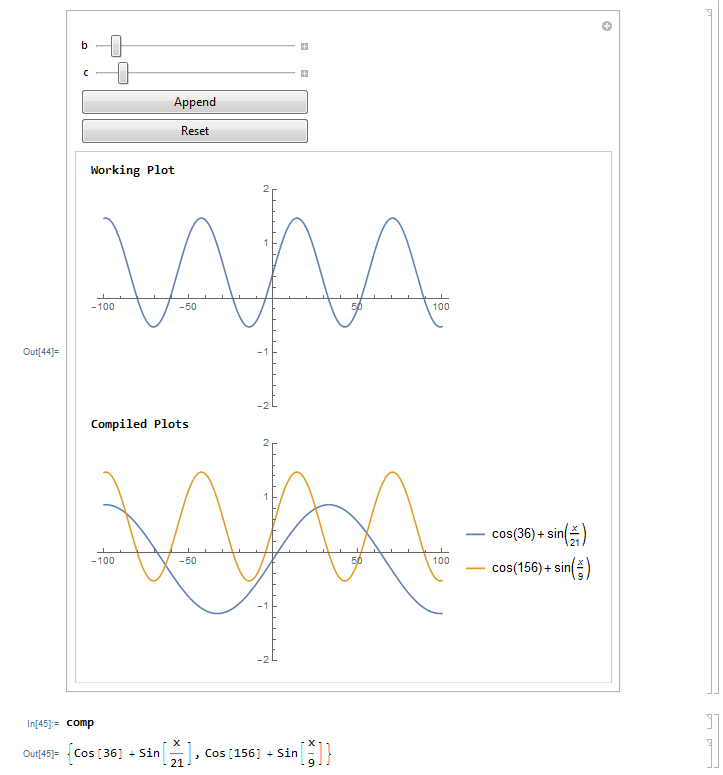
Let me know if you have more questions about my solution, or anything else that I've mentioned and I'll be happy to give more detail. I'd also be interested to see what improvements others might suggest to my answer, so I encourage everyone else to chime in as well!