Message Boards Message Boards

0
|
5858 Views
|
7 Replies
|
2 Total Likes
View groups...
Share
Share this post:

Perform Integration involving vectors, in 3D?

Posted 6 years ago
POSTED BY: Arm Mo
7 Replies

Finally, let's take B[[3]]

Bz4[x_, t_, x0_, y0_, z0_, W_, 
  T_] := -I2[T/2 + z0, t*W - y0 - W/2, x - x0] + 
  I2[z0 - T/2, t*W + y0 - W/2, x - x0]
Bz2[x_, x0_, y0_, z0_, W_, T_] := 
 Bz4[x, 1, x0, y0, z0, W, T] - Bz4[x, 0, x0, y0, z0, W, T]
Bz[x0_, y0_, z0_, W_, T_, 
  L_] := (Bz2[L/2, x0, y0, z0, W, T] - 
    Bz2[-L/2, x0, y0, z0, W, T])/(4*Pi)
Plot3D[-Bz[x, y, 20, 50, 20, 50], {x, -100, 100}, {y, -100, 100}, 
 Mesh -> None, ColorFunction -> "TemperatureMap", 
 PlotLegends -> Automatic, 
 AxesLabel -> {"x", "y", 
   "\!\(\*SubscriptBox[\(H\), \(z\)]\)/\!\(\*SubscriptBox[\(H\), \
\(c\)]\)"}, PlotRange -> All, PlotPoints -> 50, Exclusions -> None]

Z component

Attachments:

Mathematica is not a mathematician, it is a system with its limitations. Therefore, direct calculations often do not work. We must use the system to solve simple problems. But we must simplify the task ourselves. I have already solved analogous problems with vector integration. I know that a solution can be expressed in this form. Let's take B [[2]]

By4[x_, t_, x0_, y0_, z0_, W_, 
  T_] := -I2[W/2 + y0, t*T + z0 - T/2, x - x0] + 
  I2[y0 - W/2, t*T - z0 - T/2, x - x0]
By2[x_, x0_, y0_, z0_, W_, T_] := 
 By4[x, 1, x0, y0, z0, W, T] - By4[x, 0, x0, y0, z0, W, T]
By[x0_, y0_, z0_, W_, T_, 
  L_] := (By2[L/2, x0, y0, z0, W, T] - 
    By2[-L/2, x0, y0, z0, W, T])/(4*Pi)
Plot3D[-By[x, y, 20, 50, 20, 50], {x, -100, 100}, {y, -100, 100}, 
         Mesh -> None, ColorFunction -> "TemperatureMap", 
         PlotLegends -> Automatic, 
         AxesLabel -> {"x", "y", 
           "\!\(\*SubscriptBox[\(H\), \(y\)]\)/\!\(\*SubscriptBox[\(H\), \
        \(c\)]\)"}, PlotRange -> All, PlotPoints -> 50, Exclusions -> None]
![Y component ][1]
Attachments:

Try this code. There are two typical integrals through which one can express a solution

In[1]:= r0 = {x0, y0, z0};
r[1] = {x, W/2 - t*W, T/2};
r[2] = {x, -W/2, T/2 - t*T};
r[3] = {x, -W/2 + t*W, -T/2};
r[4] = {x, W/2, -T/2 + t*T};
rt = Table[D[r[i], t], {i, 1, 4}]

Out[6]= {{0, -W, 0}, {0, 0, -T}, {0, W, 0}, {0, 0, T}}

In[7]:= B = 
 Sum[Cross[rt[[i]], (r[i] - r0)]/((r[i] - r0).(r[i] - r0))^(3/2), {i, 
   1, 4}]

Out[7]= {(-((T W)/2) - 
   T y0)/((x - x0)^2 + (-(W/2) - y0)^2 + (T/2 - t T - z0)^2)^(
  3/2) + (-((T W)/2) + 
   T y0)/((x - x0)^2 + (W/2 - y0)^2 + (-(T/2) + t T - z0)^2)^(
  3/2) + (-((T W)/2) - 
   W z0)/((x - x0)^2 + (-(W/2) + t W - y0)^2 + (-(T/2) - z0)^2)^(
  3/2) + (-((T W)/2) + 
   W z0)/((x - x0)^2 + (W/2 - t W - y0)^2 + (T/2 - z0)^2)^(
  3/2), (-T x + 
   T x0)/((x - x0)^2 + (-(W/2) - y0)^2 + (T/2 - t T - z0)^2)^(3/2) + (
  T x - T x0)/((x - x0)^2 + (W/2 - y0)^2 + (-(T/2) + t T - z0)^2)^(
  3/2), (-W x + 
   W x0)/((x - x0)^2 + (-(W/2) + t W - y0)^2 + (-(T/2) - z0)^2)^(
  3/2) + (W x - 
   W x0)/((x - x0)^2 + (W/2 - t W - y0)^2 + (T/2 - z0)^2)^(3/2)}

In[23]:= Integrate[Integrate[1/(p^2 + u^2 + v^2)^(3/2), u], v]

Out[23]= ArcTan[(u v)/(p Sqrt[p^2 + u^2 + v^2])]/p

In[9]:= Integrate[Integrate[v/(p^2 + u^2 + v^2)^(3/2), u], v]

Out[9]= -ArcTanh[Sqrt[p^2 + u^2 + v^2]/u]

In[10]:= I1[p_, u_, v_] := ArcTan[(u v)/(p Sqrt[p^2 + u^2 + v^2])]/p
I2[p_, u_, v_] := -ArcTanh[Sqrt[p^2 + u^2 + v^2]/u]


In[17]:= Bx4[x_, t_, x0_, y0_, z0_, W_, 
  T_] := -(W/2 + y0)*
   I1[W/2 + y0, t*T + z0 - T/2, x - x0] + (y0 - W/2)*
   I1[y0 - W/2, t*T - z0 - T/2, x - x0] - (z0 + T/2)*
   I1[z0 + T/2, t*W - y0 - W/2, x - x0] + (z0 - T/2)*
   I1[z0 - T/2, t*W + y0 - W/2, x - x0]

In[18]:= Bx2[x_, x0_, y0_, z0_, W_, T_] := 
 Bx4[x, 1, x0, y0, z0, W, T] - Bx4[x, 0, x0, y0, z0, W, T]

In[19]:= Bx[x0_, y0_, z0_, W_, T_, 
  L_] := (Bx2[L/2, x0, y0, z0, W, T] - 
    Bx2[-L/2, x0, y0, z0, W, T])/(4*Pi)

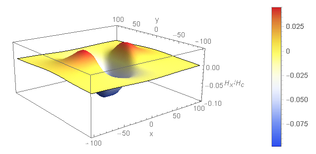
In[35]:= Plot3D[-Bx[x, y, 20, 50, 20, 50], {x, -100, 100}, {y, -100, 
  100}, Mesh -> None, ColorFunction -> "TemperatureMap", 
 PlotLegends -> Automatic, 
 AxesLabel -> {"x", "y", 
   "\!\(\*SubscriptBox[\(H\), \(x\)]\)/\!\(\*SubscriptBox[\(H\), \
\(c\)]\)"}, PlotRange -> All, PlotPoints -> 50, Exclusions -> None]

X component  of normalized magnetic ?eld at HMS = 10 for W = 50, L = 50, T = 20 nm

Attachments:
Posted 6 years ago

This looks really nice and cool. A questions though: How did you chose the functions for $I1$ and $I2$ in lines:

In[23]:= Integrate[Integrate[1/(p^2 + u^2 + v^2)^(3/2), u], v]
In[9]:= Integrate[Integrate[v/(p^2 + u^2 + v^2)^(3/2), u], v]

I kind of see that there is a $u$ function depends on $t$ (not in numerator of Sum) and $v$ function depends on $x$ (in the numerator Sum) but would like to know how did you define them to be $ - \tanh^{-1} [ \sqrt{p^2 + u^2 + v^2}/u]$ and $\tan^{-1}[\frac{\frac{u v}{p \sqrt{p^2 + u^2 + v^2}}}{p}]$ , and how did you pick coefficients for Bx4

In[17]:= Bx4[x_, t_, x0_, y0_, z0_, W_, 
  T_] := -(W/2 + y0)*
   I1[W/2 + y0, t*T + z0 - T/2, x - x0] + (y0 - W/2)*
   I1[y0 - W/2, t*T - z0 - T/2, x - x0] - (z0 + T/2)*
   I1[z0 + T/2, t*W - y0 - W/2, x - x0] + (z0 - T/2)*
   I1[z0 - T/2, t*W + y0 - W/2, x - x0]

This is good to know because I want to evaluate $H(r)$ with respect to $y$ and $z$ as well. Thanks a lot.

POSTED BY: Arm Mo
Anonymous User
Anonymous User
Posted 6 years ago

what to do depends on the answer you need

vector calculus is one way to get an answer (not the only)

for example, i could ask why not use a triple integral (but i know this may not be the area you wish to find ... in all cases)

is this for fun or do you actually have a field application you need to meet?

POSTED BY: Anonymous User
Posted 6 years ago

Let's just say I want to learn and want to follow exactly similar analytical solution. I was going to do triple integration too as you see according to my first attempt, I don't get a satisfying result from integration.

POSTED BY: Arm Mo
Reply to this discussion
Community posts can be styled and formatted using the Markdown syntax.
Reply Preview
Attachments
Remove
or Discard

Group Abstract Group Abstract