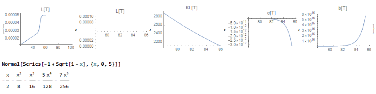
There are numerical oscillations of the function -1+Sqrt[1-x] at x->0. It is possible to use the series expansion and retain the first few terms of the series (in our example five)

(*parameter set*)
T0 = 50;
deltaHT0 = 200000;
deltaCp = 3000;
deltaHL = -10000;
Pt = 0.0001;
Lt = 0.00005;
KLT = 10^4;
R = 1.987;
f[x_] := -(x/2) - x^2/8 - x^3/16 - (5 x^4)/128 - (7 x^5)/256
K[T_] := Exp[(-deltaHT0/R)*(1/(T + 273.15) - 
      1/(T0 + 273.15)) + (deltaCp/
      R)*(Log[(T + 273.15)/(T0 + 273.15)] + (T0 + 273.15)/(T + 
         273.15) - 1)]
KL[T_] := KLT*Exp[(-deltaHL/R)*(1/(T + 273.15) - 1/(T0 + 273.15))]
b[T_] := 1 + K[T] + KL[T]*(Pt - Lt)
c[T_] := -Lt*(1 + K[T])
L[T_] := b[T]*f[4*KL[T]*c[T]/b[T]^2]/(2*KL[T])
(*track the results*)
{ Plot[{L[T]}, {T, 20, 100}, PlotLabel -> "L[T]", PlotRange -> All, 
PerformanceGoal -> "Quality"],
Plot[{L[T]}, {T, 78, 86}, PlotLabel -> "L[T]", PlotRange -> All, 
PerformanceGoal -> "Quality"],
Plot[{KL[T]}, {T, 78, 86}, PlotLabel -> "KL[T]"],
Plot[{c[T]}, {T, 78, 86}, PlotLabel -> "c[T]"],
Plot[{b[T]}, {T, 78, 86}, PlotLabel -> "b[T]"]}

Attachments:

It's most likely caused by cancellation error. To avoid this one can define all constants using exact values, then do the plot using non-machine precision so as to track and better control the error. Could all be done as below.

(*parameter set*)
T0 = 50;
deltaHT0 = 200000;
deltaCp = 3000;
deltaHL = -10000;
Pt = 1/10000;
Lt = 5/100000;
KLT = 10^4;
R = 1987/1000;
nn = 27315/100;

K[T_] = Exp[(-deltaHT0/R)*(1/(T + nn) - 1/(T0 + nn)) + (deltaCp/
       R)*(Log[(T + nn)/(T0 + nn)] + (T0 + nn)/(T + nn) - 1)];
KL[T_] = KLT*Exp[(-deltaHL/R)*(1/(T + nn) - 1/(T0 + nn))];
b[T_] = 1 + K[T] + KL[T]*(Pt - Lt);
c[T_] = -Lt*(1 + K[T]);
L[T_] = (-b[T] + Sqrt[b[T]^2 - 4*KL[T]*c[T]])/(2*KL[T]);

This will show the difference between using machine arithmetic vs bignums in the plotting.

GraphicsRow[{Plot[{L[T]}, {T, 20, 100}, PlotLabel -> "L[T]"], 
  Plot[{L[T]}, {T, 20, 100}, PlotLabel -> "L[T]", WorkingPrecision -> 20]}]