Introduction

Lattices are one of the basic mathematical structures in computational physics. Lattices are often used as discretizations of complete metric spaces since computers cannot store bona-fide real numbers, but they also sometimes assert themselves as one of the most relevant structures to take into account in hard condensed matter systems. Often this is through the phenomenon of geometric frustration: suppose you have a triangle with an Ising spin at each vertex with an antiferromagnetic interaction. Label the spins a, b, c. Suppose a is spin-up: then b wants to be spin-down, since the interaction is antiferromagnetic. But then c is in trouble: it wants to be spin-down because of its interaction with a, but wants to be spin-up because of its interaction with b. The lattice structure hence induces a six-fold ground-state degeneracy on this very simple system.

Since there are many problems involving lattices that are not trivial to implement, it would be useful for Mathematica to have some kind of built-in function for plotting data on lattices and encoding nearest-neighbor structures. This project is a first step toward that goal. The code presented here is still very much a rough draft of future hopes, but in giving it a first-go it is much clearer to me how to go about making it more efficient and modular at a second pass.

Basic Plotting

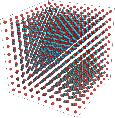
We begin by treating the body-centered cubic lattice, a Bravais lattice whose cubic unit cells consist of 1 centered atom and 8 atoms on the corners of the cube. We can summon a pair of 3D lists to represent 0's on the corners of the unit cells and 1's on the centers, then use its dimensions to produce 3D coordinates of each atom. We call the former object a "state" in analogy with physical systems.

checkerBoardState = {ConstantArray[0, {10, 10, 10}], 
   ConstantArray[1, {9, 9, 9}]};

latticePositions[
  "BodyCenteredCubic", {xrange_Integer, yrange_Integer, 
   zrange_Integer}] := Module[{corners, centers},
    corners = 
   Table[2*{i, j, k}, {i, 0, xrange - 1}, {j, 0, yrange - 1}, {k, 0, 
     zrange - 1}];
    centers = 
   Table[{1, 1, 1} + 2*{i, j, k}, {i, 0, xrange - 2}, {j, 0, 
     yrange - 2}, {k, 0, zrange - 2}];
  {corners, centers}]

checkerBoardPositions = 
  latticePositions["BodyCenteredCubic", 
   Dimensions@checkerBoardState[[1]]];

The LatticePlot function for body-centered cubic lattices takes as arguments the state, the lattice coordinates, and then two optional functions to specify properties of the spheres used to display the atoms. Here I've used Opacity and Hue to make the center atoms stand out. Radius of the spheres can also be made to depend on the state, but is defaulted at 0.35.

LatticePlot[checkerBoardState, checkerBoardPositions, 
 Opacity[(# + 1)/2] &, Hue[#/2] &]

The code for LatticePlot is not as modular or self-contained as would be desired at the moment. It handles only body-centered cubic lattices. It might be the case that there is no reason not to just construct the positions from the structure of the state in a Module. The optional functions on the state values should be implemented more carefully. Finally, since we can display multiple dimensions of data at a single point it is conceivable that the function could take several states, representing one with Hue, one with Opacity, and one with the radius of a sphere. However it's not clear to me when one would want this.

Nearest Neighbors

One of the big benefits of having lattice structures is that they implicitly define neighborhood structures (a la Moore and von Neumann) which allow us to investigate cellular automata or carry out Monte Carlo algorithms for Ising simulations.

We define functions for locating the nearest neighbors of points on the corners and in the centers using Moore and von Neumann neighborhoods respectively. The code is here for the sake of completeness, but please feel free to check out the upcoming picture for a much clearer view of what's going on.

modVec[vec_, dimensions_] := 
 MapThread[Mod[#1, #2, 1] &, {vec, dimensions}]

nearestNeighbors["BodyCenteredCubic", "Moore", 
  arrayDimensions_, {1, latticePosition__}] :=
  Catenate@{Prepend[modVec[#[[2 ;; 4]], arrayDimensions[[1]]], 
      1] & /@ (Table[{1, latticePosition} + {0}~Join~
         UnitVector[3, i], {i, 1, 3}]~Join~
      Table[{1, latticePosition} - {0}~Join~UnitVector[3, i], {i, 1, 
        3}]), Prepend[modVec[#[[2 ;; 4]], arrayDimensions[[2]]], 
      2] & /@ (Flatten[#, 2] &@
      Table[{2, latticePosition} + {0, i, j, k}, {i, -1, 0}, {j, -1, 
        0}, {k, -1, 0}])}

nearestNeighbors["BodyCenteredCubic", "von Neumann", 
  arrayDimensions_, {2, latticePosition__}] :=
Prepend[modVec[#[[2 ;; 4]], arrayDimensions[[1]]], 1] & /@ 
    Flatten[#, 2] &@
  Table[{1, latticePosition} + {0, i, j, k}, {i, 0, 1}, {j, 0, 1}, {k,
     0, 1}]

Below I've plotted the two kinds of neighborhoods. The blue dot is the dot whose neighbors we're checking for, the opaque red dots are the neighbors, and the transparent red dots are only present to show the background lattice. The neighborhood on the left with 14 red dots is a Moore neighborhood placed around each of the corner atoms. The neighborhood on the right with 8 red dots is a von Neumann neighborhood placed around each of the center atoms.

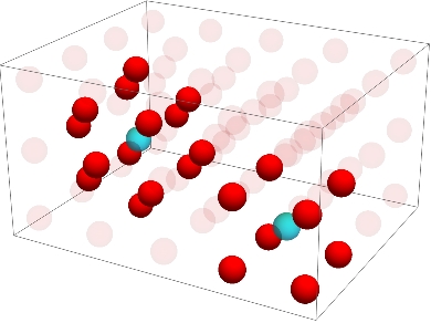
With these structures available, we can start computing the evolution of some cellular automata. We start by defining a couple functions which will give us the total value of an atom's neighbors (e.g. in the previous image, the total value of the neighbors of the left blue dot is 14, while the right blue dot is 8.)

neighborhoodTotal[state_, {1, latticePosition__}] := 
 Total[Part @@ Prepend[#, state] & /@ 
   nearestNeighbors["BodyCenteredCubic", "Moore", 
    Dimensions /@ state, {1, latticePosition}]]

neighborhoodTotal[state_, {2, latticePosition__}] := 
 Total[Part @@ Prepend[#, state] & /@ 
   nearestNeighbors["BodyCenteredCubic", "von Neumann", 
    Dimensions /@ state, {2, latticePosition}]]

Now we can define a very simple CA. This rule says if any neighbor is "on," the point of interest should turn on at the next step.

inflationRule[state_, locations_] := 
 DeleteCases[# -> If[neighborhoodTotal[state, #] > 0, 1, 0] & /@ 
   locations, _ -> 0]

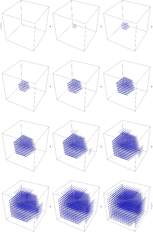
We can see this rule act on a single "seed:" in a 15 x 15 x 15 lattice there is one initial atom that is "on." We apply the rule many times and get progressively larger clumps of "on" states.

inflatedStates = 
  NestList[ReplacePart[#, inflationRule[#, locations]] &, seedState, 
   10];

LatticePlot[#, seedPositions, Hue[2 #/3] &, 
    Opacity[#/4] &, #/3 &] & /@ inflatedStates

We can get a little more fancy by running a Conway Game of Life on this lattice. Defined for completeness,

gameOfLife[starve_, crowd_, lowBirthLimit_, highBirthLimit_, state_, 
  position_] := Module[{neighborsTotal, li},
  li = position[[1]]; (*li stands for Lattice Index*)
  neighborsTotal = neighborhoodTotal[state, position]; 

  If[neighborsTotal >= crowd[[li]] \[Or] 
    neighborsTotal <= starve[[li]], position -> 0, 
   If[neighborsTotal >= lowBirthLimit[[li]] \[And] 
     neighborsTotal <= highBirthLimit[[li]], position -> 1, Nothing]]]

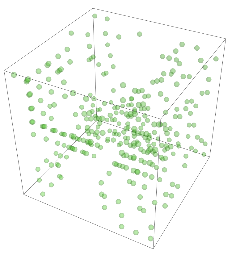
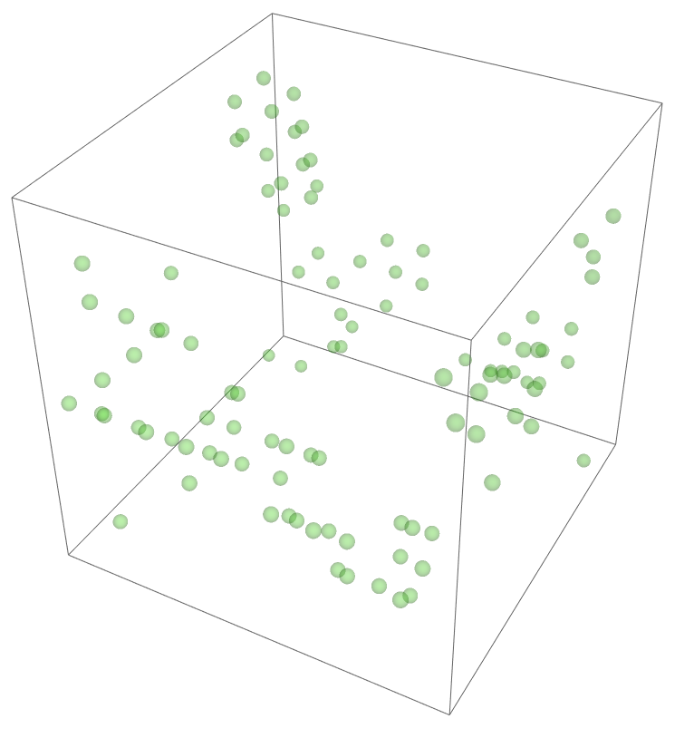
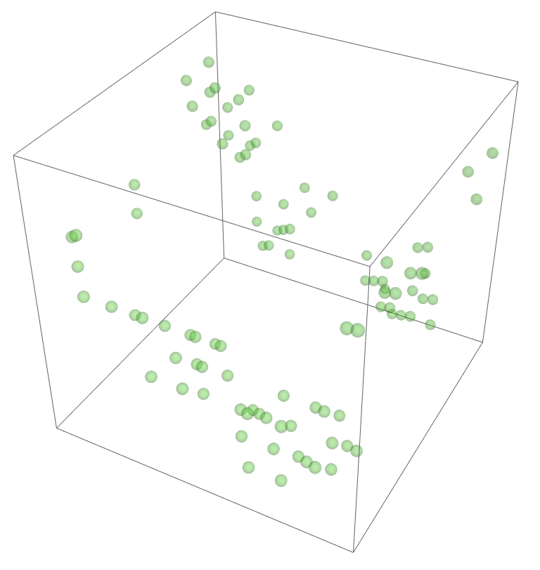
We run the game for 100 time steps, initializing on a state randomState which was generated by a p=0.2 Bernoulli trial on each entry. (I.e. an array populated randomly with 20% 1's, 80% 0's.)

lifeStates = 
  NestList[x \[Function] 
    ReplacePart[x, 
     gameOfLife[{2, 1}, {6, 4}, {4, 3}, {4, 3}, x, #] & /@ 
      randomLocations], randomState, 100];

lifePlot = 
     LatticePlot[#, randomPositions, Hue[#/3] &, 
      Opacity[#/4] &, #/3 &] & /@ 
   lifeStates;

The most legitimate way to view this is through an animation, but I guess the file was too big for my notebook to export it. Instead, please enjoy these images. Maybe if you get a good scroll going it can be like a flipbook. The final state persists to infinite time. I show it from a birds-eye-view as well to get a better look at the "still-lifes."

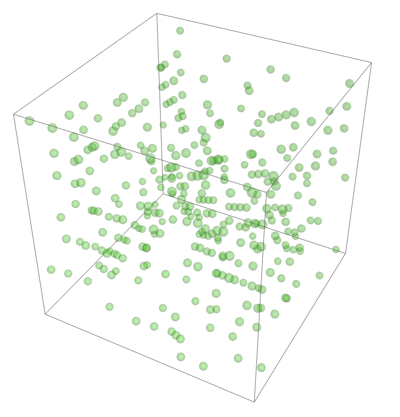
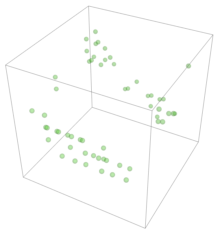
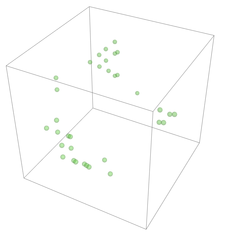
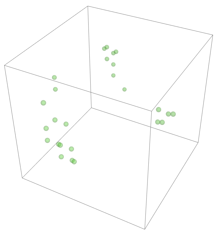
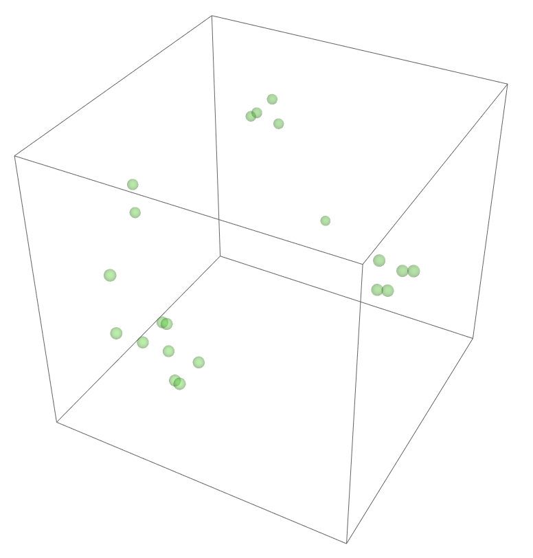
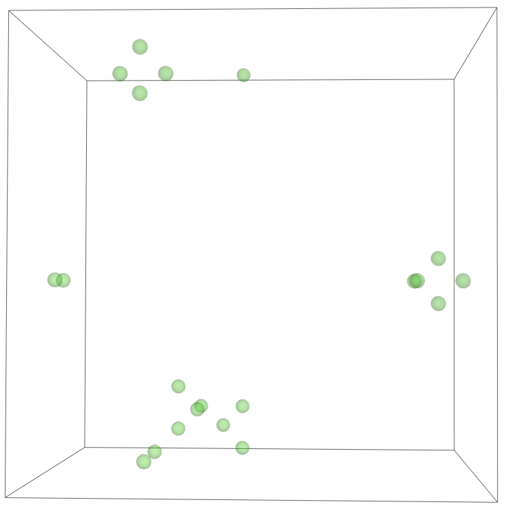
^These lads will stick around.

Conclusion and future directions

I think the most useful aspect of this project is that it is clearer now how one would go about doing this in a more systematic way. LatticePlot should look a bit more like RulePlot than it does currently, but should probably keep the feature of being able to plot arbitrary states on the lattice (if someone has highly-optimized Monte Carlo or tensor network simulations written in another language, being able to feed their data to LatticePlot directly would be very useful). It should also be more streamlined: I wouldn't be surprised if there were a method to vectorize some calculations by way of something like an image (lattice) integral a la Viola-Jones facial detection. Certainly there's a more elegant and speedier way of accessing nearest neighbors.

Something I originally wanted to do but my code was not performant enough to manage was a Monte Carlo Ising simulation. Integration with pre-built cellular automata should also be considered. Even if you have a lattice with a number of nearest-neighbors that doesn't correspond to any cellular automaton on a Z^n grid, you can always find some n large enough to truncate a totalistic automaton to your lattice of choice. The Bravais lattices should all basically follow the scheme here with minor details changed, but more exotic lattices like the Pyrochlore (causes high frustration in Heisenberg magnets) should be supported as well.

Finally, when the lattices are large (even with transparent spheres) it can be difficult to see what's going on inside. For Bravais lattices, there should in principle be a pretty good way to peer inside: a TomographyPlot function which would take in your lattice, state, and Miller indices of a plane in the lattice. The output would be a Manipulate which allowed you to see 2D slices of the lattice on the planes defined by the Miller indices.