This summer, as part of the Wolfram High School Summer Camp program, I decided to do a project analysing image dithering, and the various ways to do it. Over the course of two weeks, I learnt and understood how the algorithms work. Since resources about this process are sparse on the internet, in this post, I not only implement the algorithms, but additionally describe in detail what image dithering is and how it works.

The second part of my project was to use machine learning to classify images that originate from different image dithering algorithms.

After failing to get high accuracy with a large number of machine learning techniques, I finally came up with one that has an accuracy of about 90%.

Note that this community post is an adapted version of my computational essay. My computational essay is attached at the bottom of the post.

What is image dithering?

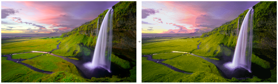
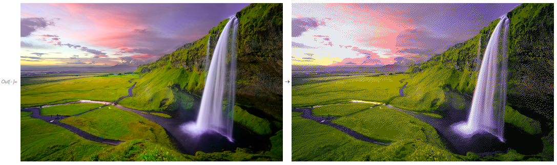
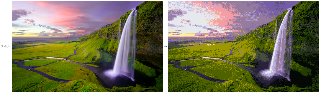
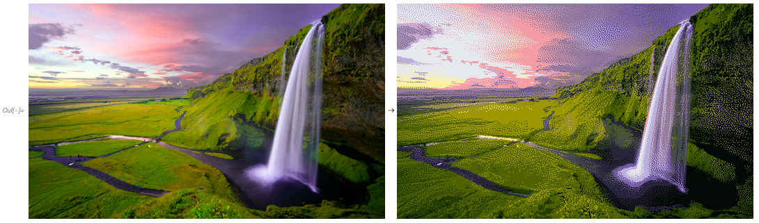
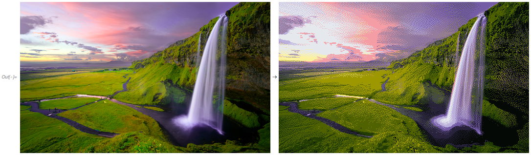
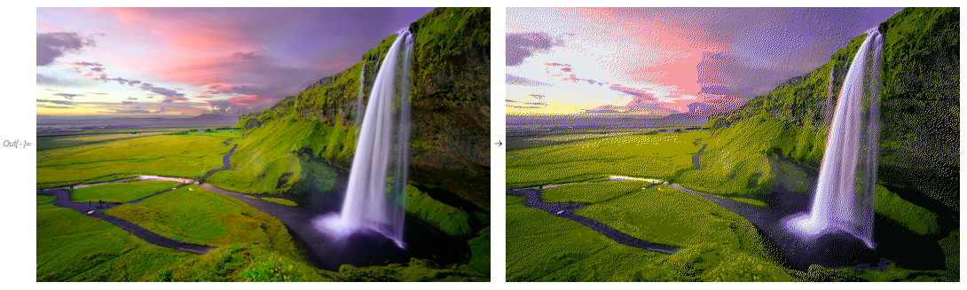
Can you tell the difference between the two images above?

The image on the right uses just 24 colours . Yet, using Floyd-Steinberg dithering, it manages to look as detailed and beautiful as the one on the left, which is using more than 16 million colours!

Let' s formally define what the aim of image dithering is :

Given an RGB image with $256^3$ colors, reduce the colour space of the image to only belong to a certain color palette.

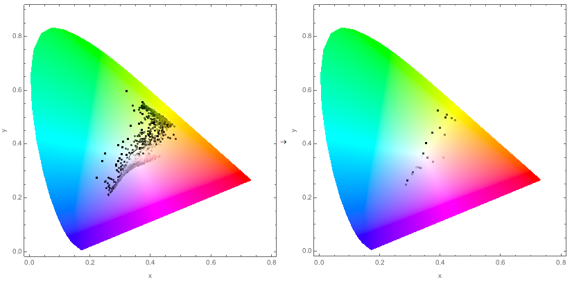
A comparison of the chromaticity plots of the above images

Color Palette

First, let us tackle the easier problem at hand. Say that we are given the option to choose our color palette, the only restriction being the number of colours in the palette. What would be the best way to obtain a color palette that is the most appropriate for an image?

Thankfully, the Wolfram Language makes this task very easy for us, as we can simply use the inbuilt function DominantColors[image, n]. For example, regarding the image above:

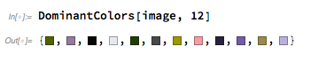
would be the most appropriate color palette with 12 colours.

Here are some visualisations of the process of choosing the color palette in 3D RGB space.

The color palette of the original image: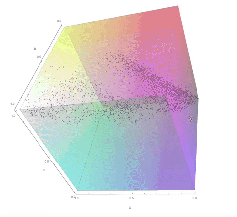

The color palette of the dithered image: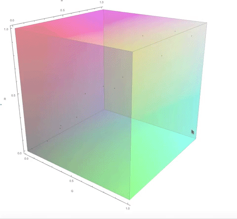

Notice how the final color palette is quite close to points on the diagonal of the cube. I go into a lot more detail about this in my computational essay.

Now, let us try to solve the main part of the problem, actually figuring out the mapping of a pixel colour to its new colour.

Naive idea

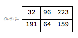
colorPallete = {0, 32, 64, 96, 128, 159, 191, 223};
pixel = {{34, 100, 222},
         {200, 50, 150}};
result = pixel;
Do [
    result[[x, y]] = First[Nearest[colorPallete, pixel[[x, y]]]];,
    {x, Length[pixel]},
    {y, Length[First[pixel]]}
  ];
Grid[result, Frame -> All, Spacings -> {1, 1}]

Extra!

I had to implement my own (but slower) version of the Wolfram function Nearest for the final functions, since pre-compiling Wolfram code to C code does not support Nearest natively. However, at the time of writing, I have heard that there is an internal project going on in Wolfram to enable support for compiling all inbuilt Wolfram function to C natively.

Better idea

As one can guess, this idea can be improved a lot. One of the important ideas is that of "smoothing". We want the transition between two objects/colours to look smoother. One way to do that would be make a gradient as the transition occurs.

However, how do you formalise a "gradient"? And how do you make a smooth one when all you have are 24 colours?

Dithering basically attempts to solves these problems.

To solve our questions, let's think about a pixel: what's the best way to make it look closest to its original colour? In the naive idea, we created some error by rounding to some nearby values.

For each pixel, let's formalise the error as:

Error diffusion

It is clear that the error should somehow be transmitted to the neighbouring elements so we can account for the error in a pixel in its neighbours. To maintain an even order of processing, let us assume that we will traverse the 2D array of pixels from the top-left corner, row-wise until we reach the bottom-right corner.

Therefore, it never makes sense to "push" the effects of an error to a cell we've already processed. Finally, let us see some ways to actually diffuse the error across the image.

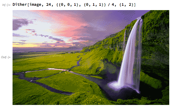
Floyd - Steinberg Dithering

In 1976, Robert Floyd and Louis Steinberg published the most popular dithering algorithm¹. The pattern for error diffusion can be described as:

diffusionFormula = {{0, 0, 7},
                    {3, 5, 1}} / 16;
diffusionPosition = {1, 2};

What does this mean?

diffusionFormula is simply a way to encode the diffusion from a pixel.

diffusionPosition refers to the position of the pixel, relative to the diffusionFormula encoding.

So, for example, an error of 2 at pixel {1, 1} translates to the following additions:

pixel[[1, 2]] += error*(7/16);
pixel[[2, 1]] += error*(3/16);
pixel[[2, 2]] += error*(5/16);
pixel[[2, 3]] += error*(1/16);

How does one come up with these weird constants?

Notice how the numerator constants are the first 4 odd numbers. The pattern is chosen specifically to create an even checkerboard pattern for perfect grey images using black and white.

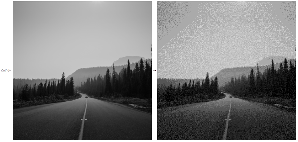
Example Grayscale image dithered with Floyd Steinberg

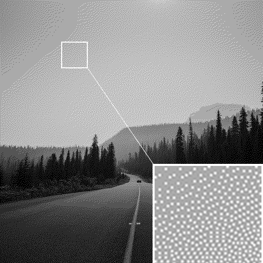
Note the checkerboard pattern in the image above.

Atkinson Dithering

Relative to the other dithering algorithms here, Atkinson's algorithm diffuses a lot less of the error to its surroundings. It tends to preserve detail well, but very continuous sections of colours appear blown out.

This was made by Bill Atkinson², an Apple employee.The pattern for error diffusion is as below :

diffusionFormula = {{0, 0, 1, 1},
                    {1, 1, 1, 0},
                    {0, 1, 0, 0}} / 8;
diffusionPosition = {1, 2};

Jarvis, Judice, and Ninke Dithering

This algorithm³ spreads the error over more rows and columns, therefore, images should be softer(in theory). The pattern for error diffusion is as below:

diffusionFormula = { {0, 0, 0, 7, 5},
                     {3, 5, 7, 5, 3},
                     {1, 3, 5, 3, 1}} / 48;
diffusionPosition = {1, 3};

The final 2 dithering algorithms come from Frankie Sierra, who published the Sierra and Sierra Lite matrices⁴ in 1989 and 1990 respectively.

Sierra Dithering

Sierra dithering is based on Jarvis dithering, so it has similar results, but it's negligibly faster.

diffusionFormula = { {0, 0, 0, 5, 3},
                     {2, 4, 5, 4, 2},
                     {0, 2, 3, 2, 0}} / 32 ;
diffusionPosition = {1, 3};

Sierra Lite Dithering

This yields results similar to Floyd-Steinberg dithering, but is faster.

diffusionFormula =  {{0, 0, 2},
                     {0, 1, 1}} / 4;
diffusionPosition = {1, 2};

Comparison

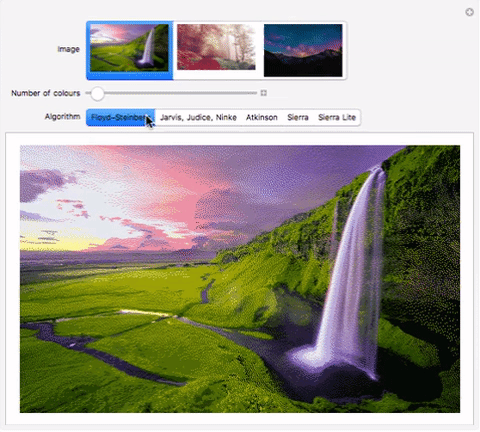
Here's an interactive comparison of the algorithms on different images:

Manipulate[
 Dither[im, c, 
  StringDelete[StringDelete[StringDelete[algo, " "], ","], 
   "-"]], {{im, image, "Image"}, {im1, im2, im3}}, {{c, 12, 
   "Number of colours"}, 2, 1024, 1}, 
 {{algo, "Floyd-Steinberg", "Algorithm"}, {"Floyd-Steinberg", 
   "Jarvis, Judice, Ninke", "Atkinson", "Sierra", "Sierra Lite"}}]

Download my computational essay to see it in action. Alternately, use the functions in the "Implementation" section to evaluate the code. im1, im2, im3 can be replaced by images. I have submitted the comparison to Wolfram Demonstrations as well, so it should be available online soon.

Side-note

Notice how the denominator in the diffusionFormula of a number of algorithms is a power of $2$? This is because division by a power of 2 is equivalent to bit-shifting the number to the right by $\log_{2}(divisor)$ bits, making it much faster than division by any other number.

Given the improvements in computer hardware, this is not a major concern anymore.

Come up with your own dithering algorithm!

I noticed that the dithering algorithms are almost the same as each other(especially the diffusionPosition).

However, I have made my functions so that you can just tweak the input arguments diffusionFormula and diffusionPosition, and test out your own functions!

Here's one I tried:

Implementation

In this section, I will discuss the Wolfram implementation, and some of the features and functions I used in my code.

applyDithering

Even though it's probably the least interesting part of the algorithm, actually applying the dithering is the most important part of the algorithm, and the one that gave me the most trouble.

I started off by writing it in the functional paradigm. With little knowledge of Wolfram, I stumbled through the docs to assemble pieces of the code. Finally, I had a "working" version of the algorithm, but there was a major problem: A $512\cdot512$ RGB image took 700 seconds for processing!

This number is way too large for an algorithm with linear time complexity in the size of input.

Fixes

Some of the trivial fixes involved making more use of inbuilt functions(for example, Nearest).

The largest problem is that the Wolfram notebook is an interpreter, not a compiler. It interprets code every time it's run. So the obvious step to optimising performance was using the Compile function in Wolfram.

But, there's a catch!

T (R1) 18 = MainEvaluate[ Hold[List][ I27, I28, T (R1) 16, R6]]
95  Element[ T (R2) 17, I20] = T (R1) 18

If you see something like the above in your machine code, your code is likely to be slow.

MainEvaluate basically means that the compiled function is calling back the kernel, which too, is a slow process.

To view the human readable form of your compiled Wolfram function, you can use:

Needs["CompiledFunctionTools`"];
CompilePrint[yourFunction]

To fix this, you need to basically write everything in a procedural form using loops and similar constructs.

The final step was RuntimeOptions -> "Speed", which trades off some integer overflow checks etc. for a faster runtime.

Find the complete code for the function below:

applyDithering = 
  Compile[{{data, _Real, 3}, {diffusionList, _Real, 
     2}, {diffusionPos, _Integer, 1}, {colors, _Real, 2}},
    Module[{lenx, leny, lenz, lenxdiff, lenydiff, error, val, 
     realLoc, closestColor, closestColordiff, res, a, diff = data, 
     diffusionFormula = diffusionList, xx, yy, curxx, curyy, 
     colorAvailable = colors, tmp, diffusionPosition = diffusionPos, 
     idx},
        {lenx, leny, lenz} = Dimensions[data];
      {lenxdiff, lenydiff} = Dimensions[diffusionFormula];
        a = data;
        res = data;
        Do[
        val = a[[x, y]];
        realLoc = {x - diffusionPos[[1]] + 1, 
       y - diffusionPos[[2]] + 1};
        closestColor = {1000000000., 1000000000., 1000000000.};
        closestColordiff = 1000000000.;
        Do[
            tmp = N[Total[Table[(i[[idx]] - val[[idx]])^2, {idx, 3}]]];
            If[tmp < closestColordiff,
              closestColordiff = tmp;
              closestColor = i;
            ];,
            {i, colorAvailable}
          ];
        error = val - closestColor;
        res[[x, y]] = closestColor;
        Do[ 
            curxx = realLoc[[1]] + xx - 1;
            curyy = realLoc[[2]] + yy - 1;
            If[curxx > 0 && curxx <= lenx && curyy > 0 && curyy <= leny,
              a[[curxx, curyy, z]] += error[[z]]*diffusionFormula[[xx, yy]]];,
            {xx, lenxdiff},
            {yy, lenydiff},
            {z, 3}
          ];,
        {x, lenx},
        {y, leny}
          ];
        Round[res]
      ],
    CompilationTarget -> "C",
    RuntimeOptions -> "Speed"
   ];

Dither

This is the main function that uses applyDithering. Their are multiple definitions of the function, one with the hardcoded values, and the other to allow one to easily implement their own dithering algorithm.

(* This is the implementation that takes the algorithm name and applies it *)

Dither[img_Image, colorCount_Integer, algorithm_String: ("FloydSteinberg" | "JarvisJudiceNinke" | 
     "Atkinson" | "Sierra" | "SierraLite")] := 
 Module[{diffusionFormulaFS, diffusionPositionFS, diffusionFormulaJJN, diffusionPositionJJN, diffusionFormulaA, 
   diffusionPositionA, diffusionFormulaS, diffusionPositionS, diffusionFormulaSL, diffusionPositionSL},
  
  (* Floyd Steinberg algorithm constants *)
    
  diffusionFormulaFS = {{0, 0, 7},
                  {3, 5, 1}} / 16;
  diffusionPositionFS = {1, 2};
  
  (* Jarvis, Judice, and Ninke algorithm constants *)
    
  diffusionFormulaJJN = {{0, 0, 0, 7, 5},
                {3, 5, 7, 5, 3},
                {1, 3, 5, 3, 1}} / 48;
  diffusionPositionJJN = {1, 3};
    
  (* Atkinson algorithm constants *)
    
  diffusionFormulaA = {{0, 0, 1, 1},
                 {1, 1, 1, 0},
                 {0, 1, 0, 0}} / 8 ;
  diffusionPositionA = {1, 2};
  
  (* Sierra algorithm constants *)
    
  diffusionFormulaS = {{0, 0, 0, 5, 3},
                 {2, 4, 5, 4, 2},
                 {0, 2, 3, 2, 0}} / 32 ;
  diffusionPositionS = {1, 3};
  
  (* Sierra Lite algorithm constants*)
    
  diffusionFormulaSL =  {{0, 0, 2},
                     {0, 1, 1}} / 4;
  diffusionPositionSL = {1, 2};

  colorAvailable = 
   Round[List @@@ ColorConvert[DominantColors[img, colorCount], "RGB"] * 255];
  Switch[algorithm,
   "FloydSteinberg", 
   Image[
       applyDithering[ImageData[RemoveAlphaChannel[img], "Byte"], diffusionFormulaFS, diffusionPositionFS, colorAvailable],
   "Byte"],
   "JarvisJudiceNinke", 
   Image[
       applyDithering[ImageData[RemoveAlphaChannel[img], "Byte"], diffusionFormulaJJN, diffusionPositionJJN, colorAvailable], 
   "Byte"],
   "Atkinson", 
   Image[
       applyDithering[ImageData[RemoveAlphaChannel[img], "Byte"], diffusionFormulaA, diffusionPositionA, colorAvailable],
   "Byte"],
   "Sierra", 
   Image[
       applyDithering[ImageData[RemoveAlphaChannel[img], "Byte"], diffusionFormulaS, diffusionPositionS, colorAvailable],
   "Byte"],
   "SierraLite", 
   Image[
       applyDithering[ImageData[RemoveAlphaChannel[img], "Byte"], diffusionFormulaSL, diffusionPositionSL, colorAvailable], 
   "Byte"]
   ]
  ];

(* This is the function that makes it easy to make your own dithering
algorithm *)

Dither[img_Image, colorCount_Integer, diffusionFormula_List, diffusionPosition_List] := Module[{},
    colorAvailable = Round[List @@@ ColorConvert[DominantColors[img, colorCount], "RGB"] * 255];
    Image[
        applyDithering[ImageData[RemoveAlphaChannel[img], "Byte"],  diffusionFormula, diffusionPosition, colorAvailable], 
    "Byte"]
   ];

Classifying images

The second part of my project involves classifying dithered images and mapping them to the algorithm they were obtained from.

This sounds like a relatively easy task for machine learning, but it turned out to be much harder. Besides, no similar research on image "metadata" has existed before, which made the task more rewarding.

I ended up creating a model which has an accuracy of more than 90%, which is reasonably good for machine learning.

If you are uninterested in the failures encountered and the details of the dataset used, please skip ahead to the section on "ResNet-50 with preprocessing".

Dataset

To obtain data, I did a web search for images with a keyword chosen randomly from a dictionary of common words.

The images obtained are then run through the five algorithms I implemented and is stored as the training data. This is to ensure that the images aren't distinguished much in terms of their actual contents, since that would interfere with learning about the dithering algorithms used in the image.

The images were allowed to use up to 24 colours which are auto-selected, as described in the section on "Color Palette".

Here is the code for downloading, applying the dithering, and re-storing the images. Note that it is not designed with re-usability in mind, these are just snippets coded at the speed of thought:

(* This function scrapes random images from the internet and stores \
them to my computer *)

getImages[out_Integer, folderTo_String] := Module[{},
  res = {};
  Do [
    Echo[x];
   l = RemoveAlphaChannel /@ 
     Map[ImageResize[#, {512, 512}] &, 
      Select[WebImageSearch[RandomChoice[WordList["CommonWords"]], 
        "Images"],
        Min[ImageDimensions[#]] >= 512 &]];
    AppendTo[res, Take[RandomSample[l], Min[Length[l], 2]]];
    Pause[10];,
    {x, out}
   ];
  MapIndexed[Export[
     StringJoin[folderTo, ToString[97 + #2[[1]]],  "-", 
      ToString[#2[[2]]], ".png"], #1] &, res, {2}]
  ]

(* This function applies the dithering and stores the image *)

applyAndStore[folderFrom_String, folderTo_String] := Module[{},
    images = FileNames["*.png", folderFrom];
    origImages = Map[{RemoveAlphaChannel[Import[#]], #} &, images];
    Map[Export[StringJoin[folderTo, StringTake[#[[2]], {66, -1}]], 
      Dither[#[[1]], 24, "Sierra"]] &, origImages]
   ];

Here are some more variable definitions and metadata about the dataset that is referenced in the following sections.

Plain ResNet-50

My first attempt was to use a popular neural net named "ResNet-50 Trained on ImageNet Competition Data,⁵ and retrain it on my training data. One of the major reasons for choosing this architecture was that it identifies the main object in an image very accurately, and is quite deep. Both these properties seemed very suitable for my use case.

However, the results turned out to be very poor. When I noticed this during the training session, I stopped the process early on. It can be speculated that the poor results were because it was trying to infer relations between the colours in the image.

Border classification

Since the borders in an image are least affected by the image dithering algorithm, and simply rounded to the closest colours, it should be easier to learn the constants of the diffusionFormula from it.

Therefore, we can pre-process an image and only use its border pixels for classification.

borderNet

Observing the aforementioned fact, I implemented a neural net which tried to work with just the borders of the image. This decreased the size of the data to $512 \cdot 4$ per image.

borderNet with just left and top border

Since my implementation of the dithering algorithms starts by applying the algorithm from the top-left corner, the pattern in the left and top borders should be even easier for the net to learn. However, this decreased the size of the data even more to $512 \cdot 2$ per image.

Both the nets failed to work very well, and had accuracies of around 20%. This was probably the case because of the lack of data for the net to actually train well enough.

Wolfram code for the net follows:

borderNet = NetChain[{
   LongShortTermMemoryLayer[100],
   SequenceLastLayer[],
   DropoutLayer[0.3],
   LinearLayer[Length@classes],
   SoftmaxLayer[]
   },
  "Input" -> {"Varying", 3},
  "Output" -> NetDecoder[{"Class", classes}]
  ]

Row and column specific classification

The aim with this approach was to first make the neural net infer patterns in the columns of the image, then combine that information and observe patterns in the rows of the image.

This didn't work very well either. The major reason for the failure was probably that the diffusion is not really as independent as the net might assume it to be.

Row and column combined classification

Building on the results of Section 2.5, the right method to do the processing seemed to be to use two separate chains, and a CatenateLayer to combine the results. For understanding the architecture, observe the NetGraph object below:

The Wolfram language code for the net is as follows:

lstmNet = NetGraph[{
   TransposeLayer[1 <-> 2],
   NetMapOperator[
    NetBidirectionalOperator[LongShortTermMemoryLayer[25], 
     "Input" -> {512, 3}], "Input" -> {512, 512, 3}],
   NetMapOperator[
    NetBidirectionalOperator[LongShortTermMemoryLayer[25], 
     "Input" -> {512, 50}], "Input" -> {512, 512, 50}],
   NetMapOperator[
    NetBidirectionalOperator[LongShortTermMemoryLayer[25], 
     "Input" -> {512, 3}], "Input" -> {512, 512, 3}],
   NetMapOperator[
    NetBidirectionalOperator[LongShortTermMemoryLayer[25], 
     "Input" -> {512, 50}], "Input" -> {512, 512, 50}],
   TransposeLayer[1 <-> 2],
   SequenceLastLayer[],
   SequenceLastLayer[],
   LongShortTermMemoryLayer[25],
   LongShortTermMemoryLayer[25],
   SequenceLastLayer[],
   SequenceLastLayer[],
   CatenateLayer[],
   DropoutLayer[0.3],
   LinearLayer[Length@classes],
   SoftmaxLayer[]
   }, {
   NetPort["Input"] -> 2 -> 3 -> 7 -> 9 -> 11,
   NetPort["Input"] -> 1 -> 4 -> 5 -> 6 -> 8 -> 10 -> 12,
   {11, 12} -> 13 -> 14 -> 15 -> 16
   },
  "Input" -> {512, 512, 3},
  "Output" -> NetDecoder[{"Class", classes}]
  ];

However, this net didn't work very well either.

The net had a somewhat unconventional architecture, and the excessive parameter count crashed the Wolfram kernel, so they had to be cut down. Ultimately, it only managed to get an accuracy rate of around 25-30%.

ResNet-50 with preprocessing

The final idea was to use pre-processing to our advantage. Dithering, in its essence, shifts the error downward and towards the right. Therefore, one way to filter the image would be to pad the image with one row of pixels at the top and one column at the left, and subtracting the padded image from the original one.

Here's an example of what that looks like:

The code for doing this to an image is as simple as:

img - ImageTake[ImagePad[img, 1], {1, 512}, {1, 512}]

Notice how the image(right side, after processing) resembles the parts with the "checkerboard" pattern described in the section "How does one come up with these weird constants?" under "Floyd - Steinberg Dithering" .

The main reason this net works well is that, even with same color palettes, the gradient of the images coming from dithering algorithms is quite different. This is because of the differences in the error diffusion, and by subtracting the padded image from the original image, we obtain a filtered version of the dithering patterns, making it easy for the neural net to spot them.

The net was trained on AWS for more than 7 hours, on a larger dataset of 1500 images.

The results outperformed my expectations, and on a test-set of more than 700 images, 300 of which were part of the original training data, it showed an accuracy rate of nearly 91%.

Here is a code of the net with details:

baseModel = 
 NetTake[NetModel["ResNet-50 Trained on ImageNet Competition Data", 
   "UninitializedEvaluationNet"], 23]

net = NetChain[{
   NetReplacePart[baseModel,
    "Input" -> NetEncoder[{"Image", {512, 512}}]],
   LinearLayer[Length@classes],
   SoftmaxLayer[]},
  "Input" -> NetEncoder[{"Image", {512, 512}, ColorSpace -> "RGB"}],
  "Output" -> NetDecoder[{"Class", classes}]
  ]

So, it's just the ResNet - 50 modified to work with $512 \cdot 512$ images.

Future Work

• Look into using machine learning for un-dithering an image.

• Look into creating new dithering algorithms that perform faster or better than the existing ones.

Notes

All images and visualisations in this post were generated in Wolfram. Their code may be seen in the computational essay attached below.

I would like to thank all the mentors, especially Greg "Chip" Hurst, Michael Kaminsky, Christian Pasquel and Matteo Salvarezza, for their help throughout the project.

Further, I would like to thank Pyokyeong Son and Colin Weller for their help during the project, and refining the essay.

The original, high resolution copies of the images are credited to Robert Lukeman, Teddy Kelley, and Sebastian Unrau on Unsplash.

References

[1] : R.W. Floyd, L. Steinberg, An adaptive algorithm for spatial grey scale. Proceedings of the Society of Information Display 17, 75-77 (1976).

[2] : Bill Atkinson, private correspondence with John Balestrieri, January 2003 (unpublished)

[3] : J. F. Jarvis, C. N. Judice and W. H. Ninke, A Survey of Techniques for the Display of Continuous Tone Pictures on Bi-level Displays. Computer Graphics and Image Processing, 5 13-40, 1976

[4] : Frankie Sierra, in LIB 17 (Developer's Den), CIS Graphics Support Forum (unpublished)

[5] : K. He, X. Zhang, S. Ren, J. Sun, "Deep Residual Learning for Image Recognition," arXiv:1512.03385 (2015)

Link to my computational essay