OK, I translated into the Wolfram Language and made a code for numerical integration. It is not possible to solve the problem analytically.
A1 = 1; A2 = 1; A3 = 1; A4 = 1; \[Epsilon] = 1; \[Kappa] = 1;
Bi = 1; Subscript[U, p] = 1; eq = {D[Subscript[\[Theta], c][x, y],
x] - A4/(\[Epsilon]*(y^2 A1 + y*A2 + A3))*
D[Subscript[\[Theta], c][x, y], y, y] == 0 ,
D[Subscript[\[Theta], s][x, y], y, y] -
Bi*(Subscript[\[Theta], s][x, y] -
Subscript[\[Theta], f][x, y]) ==
0 , \[Kappa]*D[Subscript[\[Theta], f][x, y], y, y] +
Bi*(Subscript[\[Theta], s][x, y] -
Subscript[\[Theta], f][x, y]) - \[Kappa]*Subscript[U, p]*
D[Subscript[\[Theta], f][x, y], x] == 0 };
ic = {Subscript[\[Theta], s][0, y] == 0,
Subscript[\[Theta], f][0, y] == 0,
Subscript[\[Theta], c][0, y] == 0};
bc = {DirichletCondition[ {Subscript[\[Theta], s][x, y] == 1,
Subscript[\[Theta], f][x, y] == 0,
Subscript[\[Theta], c][x, y] == 0} , y == 1],
DirichletCondition[ {Subscript[\[Theta], s][x, y] == 0,
Subscript[\[Theta], f][x, y] == 0,
Subscript[\[Theta], c][x, y] == 1} , y == 0] };
sol = NDSolve[{eq, ic, bc}, {Subscript[\[Theta], c],
Subscript[\[Theta], s], Subscript[\[Theta], f]}, {x, 0, 1}, {y, 0,
1}]
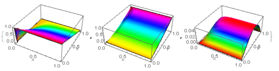
{Plot3D[Evaluate[Subscript[\[Theta], c][x, y] /. sol], {x, 0, 1}, {y,
0, 1}, Mesh -> None, ColorFunction -> Hue,
AxesLabel -> {"x", "y", ""}],
Plot3D[Evaluate[Subscript[\[Theta], s][x, y] /. sol], {x, 0, 1}, {y,
0, 1}, Mesh -> None, ColorFunction -> Hue,
AxesLabel -> {"x", "y", ""}],
Plot3D[Evaluate[Subscript[\[Theta], f][x, y] /. sol], {x, 0, 1}, {y,
0, 1}, Mesh -> None, ColorFunction -> Hue,
AxesLabel -> {"x", "y", ""}]}