NOTE: originally posted in response to: http://community.wolfram.com/groups/-/m/t/1395518
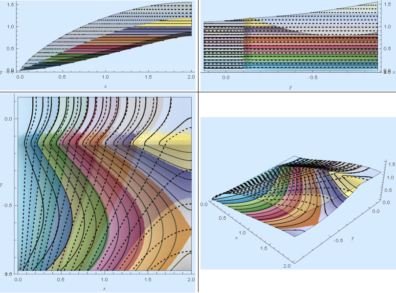
I looked at this problem as an opportunity to build some modeling and simulation skills within the Mathematica framework and to brush up on an area of physics that I have not looked at in decades. Solving a coupled convective diffusive PDE in multiple regions with discontinuous physical properties can be quite challenging. In the end, I was pleasantly surprised that I was able to "model" this system and obtain reasonable results without too much difficulty. I am documenting my path here in the hopes that someone will find it useful.
Preliminaries
I agree that there is no analytical solution to this system of coupled PDEs, and that a numerical solution is in order. The solution to the simplest convection-diffusion equation $$\rho C_pv_x\frac{\partial T}{\partial x}=k \frac{\partial^2 T}{\partial y^2}$$ for a parallel plate channel with fully developed uniform flow subjected to a uniform heat flux, Sparrow and Siegel, 1960, pg 167 showed is an infinite series. For a coupled problem, I would presume that the infinite series coefficients would depend on the infinite series coefficients of the other variables making it intractable. Ouyang et al obtain an approximate solution with an infinite series solution to a thermally developing Darcy flow in porous media.
In the FEM, it is very easy to over constrain or under constrain a system leading to bizarre results. The developers of particular tools usually have developed a framework that facilitates the construction and solving of models. It is best to operate within that framework so that we can create a functioning model with least amount of effort.
Also, in the FEM, the mesh is critcal to finding an accurate solution. In your case, you have two regions with distinct physical properties. We expect that there will be extreme changes in behavior at the interface of the two regions so we will want to resolve that area with a finer mesh.
Finally, I would recommend to start small and build complexity verifying and validating along the way.
System Description
I always like to begin with a picture of the system I am trying to model. My understanding is that there is a fluid flowing over a porous material as shown in the picture below. The flow in the x direction is assumed to be laminar parabolic flow in the fluid domain and constant uniform in the porous domain.
System Sketch
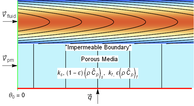
Physically, there must be an impermeable solid barrier between the two domains otherwise we would expect some flow in the Y direction. We will take advantage of this fact later.
Porous Media Domain Only
Porous Media Energy Transport Equations
As stated previously, the developers have created a framework to facilitate FEM modeling and simulation. For me, I find it often is easier to start over with that in mind than to start in the middle.
The equations below for energy transport with Local Themal Non-Equilibrium (LTNE) look formally similar to yours if we eliminate the transient and volumetric source terms shown in $\color{Red}{Red}$. If they are not, you should be able to follow the logic to develop your own.
$$\begin{gathered} {\color{Red}{(1 - \varepsilon ){\left( {\rho {{\hat C}_p}} \right)_s}\frac{{\partial {T_s}}}{{\partial t}}}}+ {\left( {\rho {{\hat C}_p}} \right)_s}\left( {{\mathbf{v}}_s \cdot \nabla {T_s}} \right) - (1 - \varepsilon )\nabla \cdot {k_s}\nabla {T_s} - {\color{Red}{(1 - \varepsilon )q_s^{'''}}} - h({T_f} - {T_s}) = 0 \qquad (1*) \\ {\color{Red}{ \varepsilon {\left( {\rho {{\hat C}_p}} \right)_f}\frac{{\partial {T_f}}}{{\partial t}}}} + {\left( {\rho {{\hat C}_p}} \right)_f}\left( {{\mathbf{v}} \cdot \nabla {T_f}} \right) - \varepsilon \nabla \cdot {k_f}\nabla {T_f} - {\color{Red}{\varepsilon q_f^{'''}}} - h({T_s} - {T_f}) = 0 \qquad (2*)\\ \end{gathered}$$
Steady-state no volumetric source terms version
$$\begin{gathered} {\left( {\rho {{\hat C}_p}} \right)_s}\left( {{\mathbf{v}}_s \cdot \nabla {T_s}} \right)- (1 - \varepsilon )\nabla \cdot {k_s}\nabla {T_s} - h({T_f} - {T_s}) = 0 \qquad (1) \\ + {\left( {\rho {{\hat C}_p}} \right)_f}\left( {{\mathbf{v}} \cdot \nabla {T_f}} \right) - \varepsilon \nabla \cdot {k_f}\nabla {T_f} - h({T_s} - {T_f}) = 0 \qquad (2)\\ \end{gathered}$$
Normally, we assume that the solid is fixed $\left(v_s={0,0}\right)$, but in this case we will retain it to use it to create an interface mixing rule. Otherwise, the solid density and heat capacity drops out of the equation.
Dimensional Analysis
When possible, I prefer to work with dimensionless equations. To make the system dimensionless, we divide the variables by characteristic variables and perform some factoring so the left hand and right hand side of the equations are dimensionless. Dimensionless temperatures and coordinates are defined as:
$$\begin{gathered} {\Theta _s} = \frac{{{T_s} - {T_0}}}{{{T_c}}};{T_s} = {T_c}{\Theta _s} + T \\ {\Theta _f} = \frac{{{T_f} - {T_0}}}{{{T_c}}};{T_f} = {T_c}{\Theta _f} + T \\ xs = \frac{x}{D};x = D \cdot xs \\ ys = \frac{y}{D};y = D \cdot ys \\ T_c = \frac{q_{0}D}{k_f} \end{gathered} $$
Making the appropriate substitutions, equations (1) and (2) become:
$$\begin{gathered} \frac{{\left( {\rho {{\hat C}_p}} \right)_s}}{{\left( {\rho {{\hat C}_p}} \right)_f}}{{\mathbf{v}}^*}_s \cdot {\nabla ^*}{\Theta _s}- \left( {1 - \varepsilon } \right)\frac{{{k_s}}}{{{k_f}}}\frac{{{\tau _{conv}}}}{{{\tau _{cond}}}}{\nabla ^*}^2{\Theta _s} - \frac{{{\tau _{conv}}}}{{{\tau _{flux}}}}({\Theta _f} - {\Theta _s}) = 0 \qquad (3) \\ {{\mathbf{v}}^*} \cdot {\nabla ^*}{\Theta _f} - \varepsilon \frac{{{\tau _{conv}}}}{{{\tau _{cond}}}}{\nabla ^*}^2{\Theta _f} - \frac{{{\tau _{conv}}}}{{{\tau _{flux}}}}({\Theta _s} - {\Theta _f}) = 0 \qquad (4) \\ \end{gathered} $$
Where the various timescales are defined by:
$$\begin{gathered} {\tau _{conv}} = \frac{D}{{{v_0}}} \\ {\tau _{cond}} = \frac{{{D^2}}}{\alpha };\alpha = \frac{{{k_f}}}{{{{\left( {\rho {{\hat C}_p}} \right)}_f}}} \\ {\tau _{flux}} = \frac{{{{\left( {\rho {{\hat C}_p}} \right)}_f}}}{h} \\ \end{gathered} $$
Consolidating the timescale ratios and noting that porosity and velocity are a function of the mesh region we are in.
$$\begin{gathered} \kappa{{\mathbf{v}}^*}_s(\Omega ) \cdot {\nabla ^*}{\Theta _s}- \left( {1 - \varepsilon (\Omega )} \right)\sigma \gamma {\nabla ^*}^2{\Theta _s} - \eta ({\Theta _f} - {\Theta _s}) = 0 \qquad (5) \\ {{\mathbf{v}}^*}(\Omega ) \cdot {\nabla ^*}{\Theta _f} - \varepsilon (\Omega )\gamma {\nabla ^*}^2{\Theta _f} - \eta ({\Theta _s} - {\Theta _f}) = 0 \qquad (6) \\ \end{gathered} $$
Where
$$\begin{gathered} \kappa = \frac{{\left( {\rho {{\hat C}_p}} \right)_s}}{{\left( {\rho {{\hat C}_p}} \right)_f}} \\ \sigma = \frac{{{k_s}}}{{{k_f}}} \\ \gamma = \frac{{{\tau _{conv}}}}{{{\tau _{cond}}}} \\ \eta = \frac{{{\tau _{conv}}}}{{{\tau _{flux}}}} \\ {{\mathbf{v}}^*} = \frac{{\mathbf{v}}}{{{v_0}}} \\ {{\mathbf{v}_s}^*} = \frac{{\mathbf{v}_s}}{{{v_0}}} \end{gathered} $$
Now, we have a system of PDEs that depend on 5 dimensionless parameters.
Neumann Boundary Condition (Flux) on Porous Boundary
When applying a flux on the porous boundary, there are different possible pathways through the fluid and solid. We must decide how to partition the heat flux. For parallel pathways, the effective conductivity is given by:
$${k_{eff}} = \left( {1 - \varepsilon } \right){k_s} + \varepsilon {k_f}$$ $$\frac{{{k_{eff}}}}{{{k_f}}} = \left( {1 - \varepsilon } \right)\sigma + \varepsilon $$
We will use this as a guide to partition the flux accordingly.
$$\begin{gathered} {x_f} = \frac{\varepsilon }{{\left( {1 - \varepsilon } \right)\sigma + \varepsilon }} \\ {q_f} = {x_f}{q_{tot}} \\ {q_s} = (1 - {x_f}){q_{tot}} \\ \end{gathered} $$
Modeling in Mathematica
With modeling, I am a firm believer that one should start simple, verify and validate the simulation results, and then build complexity. We will assume the convective diffusive heat equation has been previously validated.
Let's start with a model of the porous domain only.
Mesh Creation
I followed the tutorial in the documentation for Element Mesh Creation to generate a mesh tailored to the physical situation. You will need to load the FEM package like so
Needs["NDSolve`FEM`"]
Let's start with some definitions of a domain the is 1 unit high and 2 units long. We will also create some associations to collect surfaces and regions for clarity.
ht = 1;
len = 2;
top = ht;
bot = 0;
left = 0;
right = len;
bounds = <|inlet -> 1, hot -> 2|>;
regs = <|fluid -> 10, porous -> 20 , interface -> 15|>;
We can create a boundary mesh using the ToBoundaryMesh[] command and mark unique edges to be used as boundary conditions later. All other edges will be assigned the default boundary condtion of an insulated wall. The left edge colored $\color{Green}{Green}$ will describe the inlet condition and the bottom edge colored $\color{Red}{Red}$ will describe the heat flux condtion. All other boundaries will be the default Neumann zero flux condition.
bmesh = ToBoundaryMesh[
   "Coordinates" -> {{left, bot}(*1*), {right, bot}(*2*), {right,
      top}(*3*), {left, top}(*4*)},
   "BoundaryElements" -> {LineElement[{{1, 2}(*bottom edge*)(*1*), {4,
         1}(*left edge*)(*2*), {2, 3}(*3*), {3, 4}(*4*)}, {bounds[
        hot], bounds[inlet], 3, 3}]}];
bmesh["Wireframe"["MeshElementMarkerStyle" -> Blue,
  "MeshElementStyle" -> {Green, Red, Black}, ImageSize -> Large]]
Boundary Mesh Highlighting Special Boundaries
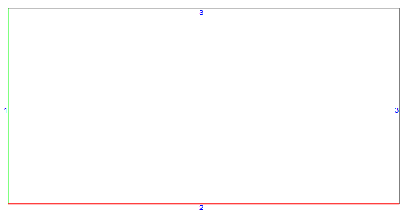
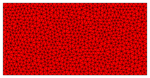
Now, we will create an element mesh that will have a $\color{Red}{Red}$ porous region with marker ID 20 (regs[porous]).
mesh = ToElementMesh[bmesh,
   "RegionMarker" -> {{{(left + right)/2, (bot + top)/2},
      regs[porous], 0.002}}];
mesh["Wireframe"["MeshElementStyle" -> {FaceForm[Red]},
  ImageSize -> Large]]
Surface Mesh
Mathematica Implementation
By investing the time we did in mesh development, we can take advantage of some facilities provided by the Wolfram developers. First, we will convert our symbols to Latin for easier reading and define some initial parameters for testing.
$$\begin{gathered} \varepsilon = eps = 0.4 \\ \sigma = s = 10 \\ \gamma = g = 2 \\ \eta = h = 0.2 \\ q_{tot} = 10 \\ v_{f} = \binom{6}{0} \\ v_{s} = \binom{0}{0} \end{gathered} $$
eps = 0.4;
s = 10;
g = 2;
h = 1/5;
mu = 5000/h;
qtot = 10;
(* Derived Parameters *)
xf = eps/((1 - eps) s + eps);
hcapfrac = 5000;
qf = xf qtot;
qs = ( 1 - xf) qtot;
p = eps;
v = {6, 0};
vs = {0, 0};
fac = 1;
We can also set our Neumann/flux boundary conditions for each state variable on the hot wall.
nvsolid = NeumannValue[qs, ElementMarker == bounds[hot]];
nvfluid = NeumannValue[qf, ElementMarker == bounds[hot]];
Likewise, we can set the inlet boundary for each state variable to 0 with Dirichlet conditions
dcsolid =
  DirichletCondition[ts[x, y] == 0, ElementMarker == bounds[inlet]];
dcfluid =
  DirichletCondition[tf[x, y] == 0, ElementMarker == bounds[inlet]];
Recasting (5) and (6) into Mathematica format (remember to put Neumann values on the right side of the equation where 0 was) we obtain:
fluideqn =
  v.Inactive[Grad][tf[x, y], {x, y}] -
    p g Inactive[Laplacian][tf[x, y], {x, y}] -
    fac h (ts[x, y] - tf[x, y]) == nvfluid;
solideqn =
  hcapfrac vs.Inactive[Grad][ts[x, y], {x, y}] - (1 -
       p) g  s Inactive[Laplacian][ts[x, y], {x, y}] -
    fac h (tf[x, y] - ts[x, y]) == nvsolid;
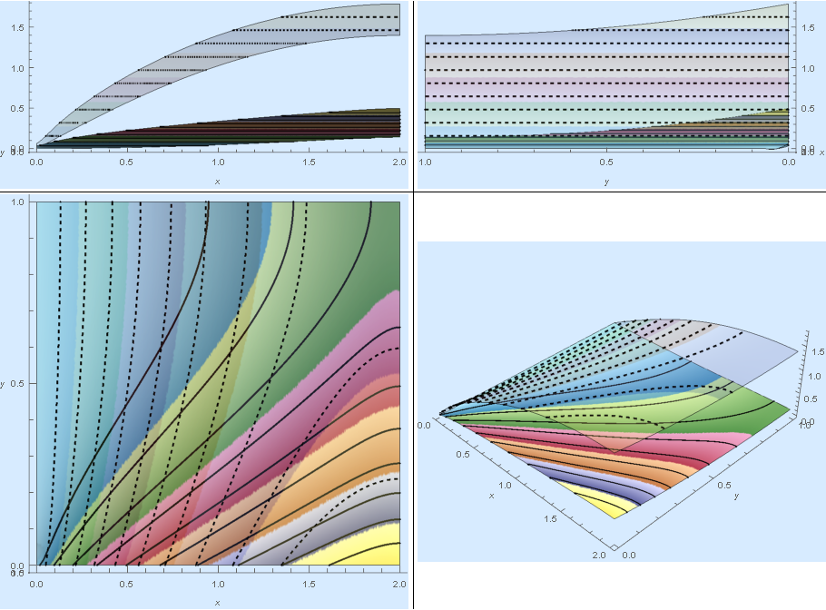
Now, we can solve on the element mesh we created earlier and do a 3D plot of the solution (Solid Temperature is translucent and has dashed lines).
ifun = NDSolveValue[{fluideqn, solideqn, dcfluid, dcsolid}, {tf,
    ts}, {x, y} \[Element] mesh];

opac = If[
   ifun[[1]][0.5, 0.5] > ifun[[2]][0.5, 0.5], {0.25, 1}, {1, 0.25}];

pltf = Plot3D[ifun[[1]][x, y], {x, y} \[Element] mesh,
   PlotRange -> All, PlotPoints -> {200, 200},
   ColorFunction -> (Directive[Opacity[opac[[1]]],
       ColorData["DarkBands"][#3]] &), MeshFunctions -> {#3 &},
   Mesh -> 10, AxesLabel -> Automatic, MeshStyle -> {Black, Thick},
   ImageSize -> Large];
plts = Plot3D[ifun[[2]][x, y], {x, y} \[Element] mesh,
   PlotRange -> All, PlotPoints -> {200, 200},
   ColorFunction -> (Directive[Opacity[opac[[2]]],
       ColorData["DarkBands"][#3]] &), MeshFunctions -> {#3 &},
   Mesh -> 10, AxesLabel -> Automatic,
   MeshStyle -> {Black, Thick, Dashed}, ImageSize -> Large];

Grid[{{Show[{pltf, plts}, ViewProjection -> "Orthographic",
    ViewPoint -> Front, ImageSize -> 450,
    Background -> RGBColor[0.84`, 0.92`, 1.`], Boxed -> False],
   Show[{pltf, plts}, ViewProjection -> "Orthographic",
    ViewPoint -> Left , ImageSize -> 450,
    Background -> RGBColor[0.84`, 0.92`, 1.`],
    Boxed -> False] }, {Show[{pltf, plts},
    ViewProjection -> "Orthographic", ViewPoint -> Top ,
    ImageSize -> 450, Background -> RGBColor[0.84`, 0.92`, 1.`],
    Boxed -> False],
   Show[{pltf, plts}, ViewProjection -> "Perspective",
    ViewPoint -> { Above, Right, Front} , ImageSize -> 450,
    Background -> RGBColor[0.84`, 0.92`, 1.`], Boxed -> False]}},
 Dividers -> Center]
Solution from Several Views
Comparison to Another Code
Because we specified a low value of $\eta$, the heat transfer between the solid and fluid phase is poor leading to a large separation of temperatures. I think the plots look nice, but do they have any basis in reality? It is always good practice to validate models versus experiments or other codes when possible.
Fortunately, I have access to other codes and can say Mathematica compares favorably as shown below ( $T_{s} = Thick\ Lines$). Having such agreement gives me confidence to continue to the more complex model.
Results from Another Code for Porous Only Domain
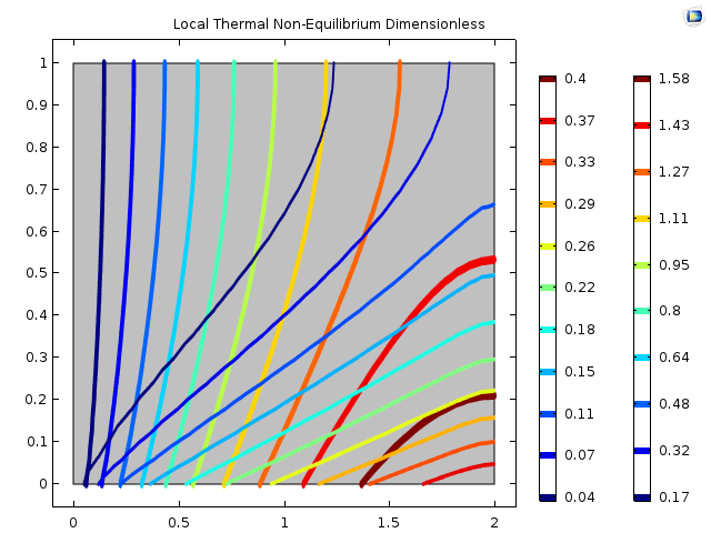
We shoud note that ${\left. T_s\neq T_f \right|_{y = top}}$ at the top of the insulated wall.
Porous Media + Fluid Domain
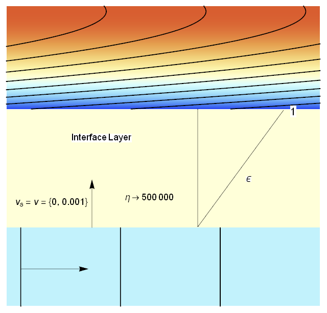
How energy is transferred through the interface between two types of media can be tricky business. Also, I don't believe that Mathematica can have internal boundary conditions currently. However, Mathematica provides other machinery to create an "interface". Recall, that I claimed that physically there must be a solid impermeable layer between the porous media and the fluid interface otherwise the porous media flow would short circuit into the fluid domain. So, let's include a thin layer in the model. This thin layer will allow us to equilibrate the solid and fluid temperatures by drastically increasing the fluid-solid heat transfer coefficient to the correct heat capacity weighted value and ramping the porosity to unity at the fluid interface so that we don't need to add another equation. A conceptual sketch is shown below.
Conceptual Model Zoomed into Interface Region
 $$\begin{gathered} \kappa{{\mathbf{v}}^*}_s(\Omega ) \cdot {\nabla ^*}{\Theta _s}- \left( {1 - \varepsilon (\Omega )} \right)\sigma \gamma {\nabla ^*}^2{\Theta _s} - -\mu(\Omega )\eta ({\Theta _f} - {\Theta _s}) = 0 \qquad (7) \\ {{\mathbf{v}}^*}(\Omega ) \cdot {\nabla ^*}{\Theta _f} - \varepsilon (\Omega )\gamma {\nabla ^*}^2{\Theta _f} -\mu(\Omega ) \eta ({\Theta _s} - {\Theta _f}) = 0 \qquad (8) \\ \end{gathered} $$
Where
$${{\mathbf{v}}^*}_s(\Omega )= \begin{Bmatrix} \binom{0}{0.001} & \Omega=Interface\\ \binom{0}{0} & True \end{Bmatrix}$$
$${{\mathbf{v}}^*}(\Omega )= \begin{Bmatrix} \binom{6}{0} & \Omega=Porous\\ \binom{20 (1 - (\frac{y}{r})^2}{0} & \Omega=Fluid\\ \binom{0}{0.001} & \Omega=Interface\\ \end{Bmatrix}$$
$$\varepsilon(\Omega )= \begin{Bmatrix} \varepsilon_0 & \Omega=Porous\\ \frac{\left(1-\varepsilon_0\right) (r+thick+y)}{thick}+\varepsilon _0 & \Omega=Interface\\ 1 & True \end{Bmatrix}$$
$$\mu(\Omega )= \begin{Bmatrix} \frac{500,000}{\eta} & \Omega=Interface\\ 1 & True \end{Bmatrix}$$
Mesh Creation for Porous, Fluid, and Coupling Interface
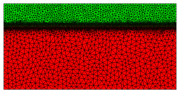
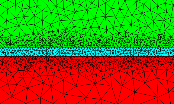
We will create a domain that is 1 unit in height by 2 units in length. The fluid ( $\color{Green}{Green}$) will occupy the top 1/4 of the domain. The interface layer ( $\color{Cyan}{Cyan}$) will be 1/40 the height. We will mark special boundaries and regions with unique IDs for boundary condition assignment and to change properties and mesh refine regions.
ht = 1;
len = 2;
r = ht/8;
top = r;
bot = r - ht;
left = 0;
right = len;
thick = ht/40;
interfacef = -r;
interfaces = -r - thick;
buffer = 1.5 thick;
(* Use associations for clearer assignment later *)
bounds = <|inlet -> 1, hot -> 2|>;
regs = <|porous -> 10, fluid -> 20, interface -> 15|>;
(* Meshing Definitions *)
(* Coordinates *)
crds = {{left, bot}(*1*), {right, bot}(*2*), {right, top}(*3*), {left,
     top}(*4*), {left, interfacef}(*5*), {right,
    interfacef}(*6*), {left, interfaces}(*7*), {right, interfaces}(*8*)};
(* Edges *)
lelms = {{1, 7}, {7, 5}, {5, 4}(*left edge*)(*1*), {1,
    2}(*bottom edge*)(*2*), {2, 8}, {8, 6}, {6, 3}, {3, 4}, {5,
    6}, {7, 8}(*3*)};
boundaryMarker = {bounds[inlet], bounds[inlet], bounds[inlet],
   bounds[hot], 3, 3, 3, 3, 3, 3}; (* 3 will be a default boundary *)
bcEle = {LineElement[lelms, boundaryMarker]};
bmesh = ToBoundaryMesh["Coordinates" -> crds,
   "BoundaryElements" -> bcEle];
bmesh["Wireframe"["MeshElementMarkerStyle" -> Blue,
  "MeshElementStyle" -> {Green, Red, Black}, ImageSize -> Large]]
(* 2D Regions *)
(* Identify Center Points of Different Material Regions *)
fluidCenter = {(left + right)/2, 0};
fluidReg = {fluidCenter, regs[fluid], 0.0005};
interfaceCenter = {(left + right)/2, (interfaces + interfacef)/2};
interfaceReg = {interfaceCenter, regs[interface], 0.00005};
porousCenter = {(left + right)/2, (bot + interfaces)/2};
porousReg = {porousCenter, regs[porous], 0.002};
meshRegs = {fluidReg, interfaceReg, porousReg};
mesh = ToElementMesh[bmesh, "RegionMarker" -> meshRegs,
   MeshRefinementFunction ->
    Function[{vertices, area}, Block[{x, y}, {x, y} = Mean[vertices];
      If[y > (interfaces + interfacef)/2 - buffer &&
        y < (interfaces + interfacef)/2 + buffer, area > 0.00005,
       area > 0.01]]]];
mesh["Wireframe"[
  "MeshElementStyle" -> {FaceForm[Green], FaceForm[Yellow],
    FaceForm[Red]}, ImageSize -> Large]]
Show[mesh[
  "Wireframe"[
   "MeshElementStyle" -> {FaceForm[Green], FaceForm[Yellow],
     FaceForm[Red]}, ImageSize -> Large]],
 PlotRange -> {{0,
    0.5}, {(interfaces + interfacef)/2 -
     4 buffer, (interfaces + interfacef)/2 + 4 buffer}}]
Boundary Mesh
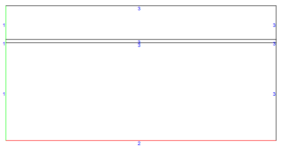
Full Mesh
Mesh Zoomed into Interface Region
NDSolve Setup and Solution
eps = 0.4;
s = 10;
g = 2;
h = 1/5;
mu = 500000/h;
qtot = 10;
xf = eps/((1 - eps) s + eps);
kappa = 500;

qf = xf qtot;
qs = ( 1 - xf) qtot;

(* Region Dependent Properties with Piecewise Functions *)
p = Evaluate[Piecewise[{{eps, ElementMarker == regs[porous]},
     {(1 - eps)/thick (y + (r + thick)) + eps,
      ElementMarker == regs[interface]},
     {1, True}}]];
v = Evaluate[Piecewise[{{{6, 0}, ElementMarker == regs[porous]},
     {{20 (1 - (y/r)^2), 0}, ElementMarker == regs[fluid]},
     {{0, 0.0001}, ElementMarker == regs[interface]}}]];
vs = Evaluate[
   Piecewise[{{{0, 0.0001}, ElementMarker == regs[interface]},
     {{0, 0}, True}}]];

(* fac increases heat transfer coefficient in interface layer *)
fac = Evaluate[If[ElementMarker == regs[interface], mu, 1]];

(* Neumann Conditions for the Hot Bottom Wall *)
nvsolid = NeumannValue[qs, ElementMarker == bounds[hot]];
nvfluid = NeumannValue[qf, ElementMarker == bounds[hot]];

(*  Dirichlet Conditions for the Left Wall *)
dcsolid =
  DirichletCondition[ts[x, y] == 0, ElementMarker == bounds[inlet]];
dcfluid =
  DirichletCondition[tf[x, y] == 0, ElementMarker == bounds[inlet]];

(* Balance Equations for Fluid and Solid Temperature *)
fluideqn =
  v.Inactive[Grad][tf[x, y], {x, y}] -
    p g Inactive[Laplacian][tf[x, y], {x, y}] -
    fac h (ts[x, y] - tf[x, y]) == nvfluid;
solideqn =
  kappa vs.Inactive[Grad][ts[x, y], {x, y}] - (1 - p) g  s Inactive[
       Laplacian][ts[x, y], {x, y}] - fac h (tf[x, y] - ts[x, y]) ==
   nvsolid;

ifun = NDSolveValue[{fluideqn, solideqn, dcfluid, dcsolid}, {tf,
    ts}, {x, y} \[Element] mesh];

(* Set opacity for higher temperature to be translucent so we can see \
the layer below *)
opac = If[
   ifun[[1]][0.5, (-r + bot)/2] > ifun[[2]][0.5, (-r + bot)/2], {0.25,
     1}, {1, 0.25}];

(* Plots *)
pltf = Plot3D[ifun[[1]][x, y], {x, y} \[Element] mesh,
   PlotRange -> All, PlotPoints -> {200, 200},
   ColorFunction -> (Directive[Opacity[opac[[1]]],
       ColorData["DarkBands"][#3]] &), MeshFunctions -> {#3 &},
   Mesh -> 18, AxesLabel -> Automatic, MeshStyle -> {Black, Thick},
   ImageSize -> Large];
plts = Plot3D[ifun[[2]][x, y], {x, y} \[Element] mesh,
   PlotRange -> All, PlotPoints -> {200, 200},
   ColorFunction -> (Directive[Opacity[opac[[2]]],
       ColorData["DarkBands"][#3]] &), MeshFunctions -> {#3 &},
   Mesh -> 18, AxesLabel -> Automatic,
   MeshStyle -> {Black, Thick, Dashed}, ImageSize -> Large];
Grid[{{Show[{pltf, plts}, ViewProjection -> "Orthographic",
    ViewPoint -> Front, ImageSize -> 400,
    Background -> RGBColor[0.84`, 0.92`, 1.`], Boxed -> False],
   Show[{pltf, plts}, ViewProjection -> "Orthographic",
    ViewPoint -> Left , ImageSize -> 400,
    Background -> RGBColor[0.84`, 0.92`, 1.`],
    Boxed -> False] }, {Show[{pltf, plts},
    ViewProjection -> "Orthographic", ViewPoint -> Top ,
    ImageSize -> 400, Background -> RGBColor[0.84`, 0.92`, 1.`],
    Boxed -> False],
   Show[{pltf, plts}, ViewProjection -> "Perspective",
    ViewPoint -> { Above, Right, Front} , ImageSize -> 400,
    Background -> RGBColor[0.84`, 0.92`, 1.`], Boxed -> False]}},
 Dividers -> Center]
Full Model Porous + Interface + Fluid

Comparison to Another Code
Again, as shown below, the Mathematica solution compares qualitatively favorably to another code. The contour plots have similar shapes but Mathematica has about 40% higher temperatures, which could indicate that I dropped or added a $\varepsilon$ somewhere in the setup of the other code, but a detailed debugging is probably in order. The implementation in the other code is slightly different due to different capabilities which I will elaborate. In the other code, the interface layer is a just a high thermal conductivity solid. I am able to set the porous-solid interface temperature to be equal to the porous temperature (solid-fluid bulk mix temperature).
Another Code Full Model Porous + Interface + Fluid
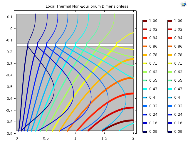
Finally, because I know that I can set an interface boundary condition in the other code, I can remove the interface region and set the fluid boundary condition to the porous mean temperature and judge the effect. As shown in the image below, it probably would not change conclusions much.
Another Code Full Model Porous + Fluid No Interface
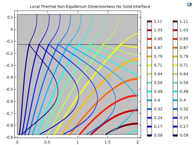
Future Enhancements
After looking at the documentation and reading the literature, I should recast the equations to conform to the coefficient form of the PDE so that I could additionally scale the $x$ coordinate by the Péclet number. This would allow for easier comparison to literature and keep a more reasonable aspect ratio for the domain.
$$\nabla \cdot\left( { - \mathbf{c}\nabla u - \alpha u + \gamma } \right) + \beta \cdot\nabla u + au - f = 0$$
Summary
- An exact analytical solution to an LTNE problem coupled to a fluid domain seems improbable.
- Mathematica
- Currently, I don't think interface BCs can be defined in the FEM framework.
- Does provide meshing features that allow the construction of an interface with finite thickness that might be used a workaround to this limitation.
- Results
- Porous Media Only Domain.
- Quite easy to setup a mesh and identify unique boundaries and regions.
- Straightforward to translate our system of PDEs created by hand into equations suitable for Mathematica.
- Relatively easy to post process results using examples from documentation.
- Solution compares favorably to another PDE code.
- Combined Porous Media--Interface--Fluid Domains
- Quite easy to setup a mesh with appropriate refinement and identify unique boundaries and regions.
- Straightforward to translate our system of PDEs created by hand into equations suitable for Mathematica.
- Relatively easy to post process results using examples from documentation.
- Solution compares qualitatively favorably to another PDE code.
- Additional study/debugging will be required to fully harmonize the results.
- Could be a simple matter of missing a parameter or something deeper.
- Conclusion
- A prototype of a simple LTNE model was developed in Mathematica.
- In modeling, there are many ways to skin a cat and this is just one possible way that produces a solution in a resonable period. More elegant solutions are welcome.
- Additional model development and validation is necessary.
- Mathematica provides enough features and tools that you can get close to what you need with some imagination.
Attachment
The attached notebook has the complete code to produce a solution to study and modify as one sees fit. I did recast the equations into coefficient form because that appears to be better practice. Storing the solution will increase notebook size >100MB.
 Attachments: