Message Boards Message Boards

Solve the Nonlinear Schroedinger Equation with NDSolve?

I’m trying to solve the a special form of the Nonlinear Schroedinger Equation using NDSolve (see file attached) and run into the problem of “Warning: scaled local spatial error estimate of …”. This is presumably due to the low resolution along the tau-axis, while increasing this number leads to a massive increase in simulation time.

For instance if I set MinPoints=600, simulation time is 0.47s, while if MinPoints=2000, simulation time increases to 80s, while the warning is still present.

Does any one of you have experience in setting up NDSolve such that good solutions are obtained while maintaining a reasonable simulation speed, particular in the case of the Nonlinear Schrödinger Equation?

What is actually the meaning of “MaxStepSize”?

Thanks in advance. Markus

Attachments:
POSTED BY: Markus Schmidt
16 Replies

Markus, how did you find constants $\delta3, \delta4, NS$?

The constants are a result of the physical problem that I'm trying to solve. I'm investigating temporal solitons in optical fibers (i.e., non-dispersive solitons in the time domain), and the dispersion of the mode of interest imposes the higher-order terms in the Nonlinear Schrödinger Equation. The actual values are associated with the fiber used and can changed if another configuration of fiber and pulse are used. Typically, these values are varied to find interesting fiber structures.

POSTED BY: Markus Schmidt

To test the effectiveness of all algorithms, I used a 1D type solution $Us[\tau, \xi]=Us[\tau-\xi]$ as the initial and boundary conditions. Unfortunately, all the algorithms turned out to be ineffective in the sense that the error in reproducing the 1D solution was in all cases higher than 0.5%.This is due to the fact that waves arise in the 2D solution, which are not present in the 1D solution. There were in all cases, a system error warning

NDSolve::mxsst: Using maximum number of grid points 10000 allowed by the MaxPoints or MinStepSize options for independent variable \[Tau].


NDSolve::eerr: Warning: scaled local spatial error estimate of 14.571949730562471` at \[Xi] = 1.` in the direction of independent variable \[Tau] is much greater than the prescribed error tolerance. Grid spacing with 10001 points may be too large to achieve the desired accuracy or precision. A singularity may have formed or a smaller grid spacing can be specified using the MaxStepSize or MinPoints method options.

When using the "MethodOfLines" there is a message

DynamicNDSolve::ibcinc: Warning: boundary and initial conditions are inconsistent.

Although the same boundary and initial conditions are consistent when using the automatic method. Consider an example

\[Delta]3 = 0.00404040404040404`30;
\[Delta]4 = -4.2087542087542085`30*^-6;
NS = 4.483404754211932`30;
NS2 = 20.100918190090154388694371172624`30;
\[Xi]max = 1;
\[Tau]max = 1;
x0 = -5/2; xm = 5/2;
q = 1.3862943611198906`30;
eq0 = {-I NS2 Abs[F[x]]^2 F[x] - Derivative[1][F][x] - 
    1/2 I (F^\[Prime]\[Prime])[x] - \[Delta]3 
\!\(\*SuperscriptBox[\(F\), 
TagBox[
RowBox[{"(", "3", ")"}],
Derivative],
MultilineFunction->None]\)[x] - I \[Delta]4 
\!\(\*SuperscriptBox[\(F\), 
TagBox[
RowBox[{"(", "4", ")"}],
Derivative],
MultilineFunction->None]\)[x]};
Us1 = NDSolveValue[{eq0 == 0, F[x0] == 1, F'[x0] == 0, 
    F''[x0] == -2*q, F'''[x0] == 0}, F, {x, x0, xm}, 
   WorkingPrecision -> 30, MaxSteps -> 10^6];

Plot[Abs[Us1[\[Tau]]], {\[Tau], x0, xm}, Frame -> True, 
 PlotStyle -> Darker[Blue], PlotRange -> All, Filling -> Bottom]
eqs = {D[Us[\[Tau], \[Xi]] , \[Xi]] - 
     I/2*D[Us[\[Tau], \[Xi]], {\[Tau], 2}] - \[Delta]3*
      D[Us[\[Tau], \[Xi]], {\[Tau], 3}] - 
     I*\[Delta]4*D[Us[\[Tau], \[Xi]], {\[Tau], 4}] - 
     I*NS2*Abs[Us[\[Tau], \[Xi]]]^2*Us[\[Tau], \[Xi]] == 0}; 
bc = {Us[\[Tau]max, \[Xi]] == Us1[\[Tau]max - \[Xi]], 
   Us[-\[Tau]max, \[Xi]] == Us1[-\[Tau]max - \[Xi]], 
   Derivative[1, 0][Us][\[Tau]max, \[Xi]] == 
    Derivative[1][Us1][\[Tau]max - \[Xi]], 
   Derivative[1, 0][Us][-\[Tau]max, \[Xi]] == 
    Derivative[1][Us1][-\[Tau]max - \[Xi]]};
ic = {Us[\[Tau], 0] == Us1[\[Tau]]};
sol = NDSolve[Join[eqs, ic, bc], 
    Us, {\[Tau], -\[Tau]max, \[Tau]max}, {\[Xi], 0, \[Xi]max}, 
    MaxSteps -> 10^6];
Plot3D[Abs[Us[\[Tau], \[Xi]]] /. 
  Last[sol], {\[Tau], -\[Tau]max, \[Tau]max}, {\[Xi], 0, \[Xi]max}, 
 Mesh -> None, ColorFunction -> Hue, PlotRange -> All]

1D and 2D solutions fig1 Difference of 1D and 2D solutions

{Plot[{Abs[Us1[\[Tau] - .5]] - Abs[Us[\[Tau], .5]] /. 
    Last[sol]}, {\[Tau], -\[Tau]max, \[Tau]max}], 
 Plot[{Arg[Us1[\[Tau] - .5]] - Arg[Us[\[Tau], .5]] /. 
    Last[sol]}, {\[Tau], -\[Tau]max, \[Tau]max}, PlotRange -> All]}

fig2 Difference of 1D and 2D solutions in the case of the most optimal method out of 8 studied

sol = NDSolve[Join[eqs, ic, bc], 
   Us, {\[Tau], -\[Tau]max, \[Tau]max}, {\[Xi], 0, \[Xi]max}, 
   Method -> {"MethodOfLines", 
     "SpatialDiscretization" -> {"TensorProductGrid", 
       "MinPoints" -> 40, "MaxPoints" -> 2000, 
       "DifferenceOrder" -> 4}}];

fig3

The method that Markus used allows to reduce the amplitude of parasitic waves by an order of magnitude. Although the time spent in this method is 6.5 times more than in the optimal method. Difference of 1D and 2D solutions in the case of Markus method.

sol = NDSolve[Join[eqs, ic, bc], 
  Us, {\[Tau], -\[Tau]max, \[Tau]max}, {\[Xi], 0, \[Xi]max}, 
  Method -> {"MethodOfLines", 
    "SpatialDiscretization" -> {"TensorProductGrid", 
      "MinPoints" -> 2000, "DifferenceOrder" -> 2}}, 
  PrecisionGoal -> 5, AccuracyGoal -> 5, MaxSteps -> \[Infinity]]

fig4

Hi Markus,

Could you provide an inefficient, but accurate, solution pointing out the key required features to capture? When I look at your solutions, it is clear that the low resolution case missed many spikey features. Do you care about those features? Does that imply that the high resolution solution is accurate? There is no point trying to speed up an inaccurate solution. Is there an area that you would like to resolve? Most of the action appears to be centered around low absolute $\tau$. What are you trying to resolve and has your approach resolved it or do we need to refine further?

I used the following plot functions to view your cases of MinPoints->600 and 2000, respectively.

plt = Plot3D[
  Evaluate[Abs[Us[\[Tau], \[Xi]]] /. 
    Last[sol]], {\[Tau], -\[Tau]max, \[Tau]max}, {\[Xi], 0, \[Xi]max},
   PlotPoints -> {100, 100}, MaxRecursion -> 4, 
  ColorFunction -> 
   Function[{x, y, z}, Directive[ColorData["DarkBands"][z]]], 
  ColorFunctionScaling -> False, MeshFunctions -> {#3 &}, Mesh -> 50, 
  PlotRange -> All, Boxed -> False, Axes -> False, ImageSize -> Large]

sz = 300;
Grid[{{Show[{plt}, ViewProjection -> "Orthographic", 
    ViewPoint -> Front, ImageSize -> sz, 
    Background -> RGBColor[0.84`, 0.92`, 1.`], Boxed -> False], 
   Show[{plt}, ViewProjection -> "Orthographic", ViewPoint -> Right, 
    ImageSize -> sz, Background -> RGBColor[0.84`, 0.92`, 1.`], 
    Boxed -> False]}, {Show[{plt}, ViewProjection -> "Orthographic", 
    ViewPoint -> Top, ImageSize -> sz, 
    Background -> RGBColor[0.84`, 0.92`, 1.`], Boxed -> False], 
   Show[{plt}, ViewProjection -> "Perspective", 
    ViewPoint -> {Above, Right, Front}, ImageSize -> sz, 
    Background -> RGBColor[0.84`, 0.92`, 1.`], Boxed -> False]}}, 
 Dividers -> Center]

Hi Res Grid

enter image description here I indicated a "Hair Line" on the figure. I would have assumed it was a simulation artifact, but you might be trying to resolve it given your statement about "fission", but how would one know? I zoomed in on the right and left side.

Hi Res Right Zoom

enter image description here

Hi Res Left Zoom

enter image description here

Low Res Grid

enter image description here

If we zoom in on the $\tau$ scale, the instability for the low resolution is clearer.

Hi Res Zoom

enter image description here

Low Res Zoom

enter image description here This may look like fission, but it is probably numerical. If we look at the underside of the Hi Res Zoom, we see some very sharp spikes that the solver needs to detect while solving before it can resolve. enter image description here

You can view the adaptive mesh actions the solver took to resolve the spikes by selecting the Mesh->All option in Plot3D. If we zoom in on a spike, we can see the refinements.

enter image description here

In the low res case, the spike probably existed within a mesh element.

Applying a Window Function

For $\tau>5$, the Gaussian function is numerical insignificant relative to your range as alluded to by Alexander. Could we apply a window function using (UnitStep[4-$\tau>5$]-UnitStep[4+$\tau>5$])? When I do that with DifferenceOrder->4, all sorts of splitting happens (4 distinct peaks). Is that real? Also, the solution on my machine is about 3.5 x faster (20 seconds) than without the window function.

Clear["`*"]; ClearAll; ClearAll["Global\[OpenCurlyQuote]*"]; \
Remove["Global`*"];
SetDirectory[NotebookDirectory[]];

\[Delta]3 = 0.00404040404040404;
\[Delta]4 = -4.2087542087542085*^-6;
NS = 4.483404754211932;

\[Xi]max = 1;
\[Tau]max = 30;

Us1[\[Tau]_] = 
  Exp[-1.3862943611198906*\[Tau]^2] (UnitStep[5 - \[Tau]] + 
     UnitStep[5 + \[Tau]]);
Plot[Us1[\[Tau]], {\[Tau], -\[Tau]max, \[Tau]max}, Frame -> True, 
  PlotStyle -> Darker[Blue], PlotRange -> All, Filling -> Bottom];
eqs = {D[Us[\[Tau], \[Xi]] , \[Xi]] - 
     I/2*D[Us[\[Tau], \[Xi]], {\[Tau], 2}] - \[Delta]3*
      D[Us[\[Tau], \[Xi]], {\[Tau], 3}] - 
     I*\[Delta]4*D[Us[\[Tau], \[Xi]], {\[Tau], 4}] - 
     I*NS^2*Abs[Us[\[Tau], \[Xi]]]^2*Us[\[Tau], \[Xi]] == 0}; 
bc = {Us[\[Tau]max, \[Xi]] == 0, 
   Us[-\[Tau]max, \[Xi]] == 
    0, (D[Us[\[Tau], \[Xi]], {\[Tau], 1}] /. \[Tau] -> \[Tau]max) == 
    0, (D[Us[\[Tau], \[Xi]], {\[Tau], 1}] /. \[Tau] -> -\[Tau]max) == 
    0};
ic = {Us[\[Tau], 0] == Us1[\[Tau]]};
Print["seconds to obtain solution: ",
  time = AbsoluteTiming[
     Monitor[
       sol = 
        NDSolve[Join[eqs, ic, bc], 
         Us, {\[Tau], -\[Tau]max, \[Tau]max}, {\[Xi], 0, \[Xi]max}, 
         EvaluationMonitor :> (\[Xi]current = \[Xi]), 
         Method -> {"MethodOfLines", 
           "SpatialDiscretization" -> {"TensorProductGrid", 
             "MinPoints" -> 2000, "DifferenceOrder" -> 4}}, 
         PrecisionGoal -> 5, AccuracyGoal -> 5, 
         MaxSteps -> \[Infinity]], 
       "current \[Xi] (\!\(\*SubscriptBox[\(\[Xi]\), \(max\)]\)=" <> 
        ToString[\[Xi]max] <> "): " <> ToString[ \[Xi]current]];][[
    1]]] ;
Print["grid points along {\[Tau],\[Xi]}-directions: ", 
  Length /@ InterpolatingFunctionCoordinates[Us /. sol[[1]]]];

(UnitStep[4-$\tau$]-UnitStep[4+$\tau$])

enter image description here

(UnitStep[5-$\tau$]-UnitStep[5+$\tau$])

enter image description here There seems to be minor change going from 4 to 5 on the window function, indicating little sensitivity in that range.

Zoomed

enter image description here

(UnitStep[6-$\tau$]-UnitStep[6+$\tau$])

enter image description here

Here is an animation along the $\xi$ coordinate for an alternative visualization.

enter image description here

Summary

We may or may not be making progress. Adding a window function when the Gaussian becomes insignificant, seems to induce splitting. We will need some more definition from you about your requirements and what the expected results are to make any additional progress. If we are on the right path, then a 20 seconds solve time should enable 4000 simulations per day.

POSTED BY: Tim Laska

Hi Tim.

Resolution is really critical, since self-consistant solutions (solitons) decay artifically. The hair lines you indicated are not related to a real world system.

I have attached two files, where the first cell is my code and the second cell is your code with the special definition of the U-function:

  1. "test file-delta3=0.00": This file (delta=0) shows you the real solution in the first cell of the notebook. The solution breatch but are stable, which is a so-called higher order soliton. Your code, in contrast, delivery unphysical solutions, which I think comes from the input function being artifically put to zero. I think that your code is good, but just the initial conditions is different to what can physically be provided in a real work system

  2. "test file-delta3=0.04": In this case (delta=0.04), the soliton undergoes fission at a particular distance, as you can see in my code. Here, I could not reach a solution with your code in a reasonable time.

This really shows that the solution of the Nonlinear Schrödinger Equations is really sensitive to the initial condition, which is a characteristicam of nonlinear systems. Therefore a modifcation of the initial conditions is not good. In any case, I still have serious problems with the simulation time, since for particular (and from my point of view non-systematic) combinations of solver setting simulation can get very long. Do you have another idea?

Thanks,

Markus

POSTED BY: Markus Schmidt

Hi Markus,

I am about to head out for the evening, but here is an odd difference order attempt, which the documentation advise against, but it is fast (<6 seconds on my machine).

\[Delta]3 = 0;
\[Delta]4 = 0;
NS = 4;

\[Xi]max = 0.6;
\[Tau]max = 10;

Us1[\[Tau]_] = Exp[-1.3862943611198906*\[Tau]^2];
Plot[Us1[\[Tau]], {\[Tau], -\[Tau]max, \[Tau]max}, Frame -> True, 
  PlotStyle -> Darker[Blue], PlotRange -> All, Filling -> Bottom];
eqs = {D[Us[\[Tau], \[Xi]] , \[Xi]] - 
     I/2*D[Us[\[Tau], \[Xi]], {\[Tau], 2}] - \[Delta]3*
      D[Us[\[Tau], \[Xi]], {\[Tau], 3}] - 
     I*\[Delta]4*D[Us[\[Tau], \[Xi]], {\[Tau], 4}] - 
     I*NS^2*Abs[Us[\[Tau], \[Xi]]]^2*Us[\[Tau], \[Xi]] == 0}; 
bc = {Us[\[Tau]max, \[Xi]] == 0, 
   Us[-\[Tau]max, \[Xi]] == 
    0, (D[Us[\[Tau], \[Xi]], {\[Tau], 1}] /. \[Tau] -> \[Tau]max) == 
    0, (D[Us[\[Tau], \[Xi]], {\[Tau], 1}] /. \[Tau] -> -\[Tau]max) == 
    0};
ic = {Us[\[Tau], 0] == Us1[\[Tau]]};
Print["seconds to obtain solution: ",
  time = AbsoluteTiming[
     Monitor[
       sol = 
        NDSolve[Join[eqs, ic, bc], 
         Us, {\[Tau], -\[Tau]max, \[Tau]max}, {\[Xi], 0, \[Xi]max}, 
         EvaluationMonitor :> (\[Xi]current = \[Xi]), 
         Method -> {"MethodOfLines", 
           "SpatialDiscretization" -> {"TensorProductGrid", 
             "MinPoints" -> 2000, "DifferenceOrder" -> 5}}(*,
         PrecisionGoal\[Rule]5,AccuracyGoal\[Rule]5,
         MaxSteps\[Rule]\[Infinity]*)], 
       "current \[Xi] (\!\(\*SubscriptBox[\(\[Xi]\), \(max\)]\)=" <> 
        ToString[\[Xi]max] <> "): " <> ToString[ \[Xi]current]];][[
    1]]] ;
Print["grid points along {\[Tau],\[Xi]}-directions: ", 
  Length /@ InterpolatingFunctionCoordinates[Us /. sol[[1]]]];
U2[\[Tau]_, \[Xi]_] = Us[\[Tau], \[Xi]] /. sol[[1]];
UAbs[\[Tau]_, \[Xi]_] = U2[\[Tau], \[Xi]] // Abs;
\[Tau]1 = -10.0; \[Tau]2 = 10.0; \[Xi]1 = 0.0; \[Xi]2 = \[Xi]max;
DensityPlot[
  UAbs[\[Tau], \[Xi]], {\[Tau], \[Tau]1, \[Tau]2}, {\[Xi], \[Xi]1, \
\[Xi]2}, PerformanceGoal -> "Quality", 
  ColorFunction -> "BlueGreenYellow", PlotRange -> All, 
  FrameLabel -> {"\[Tau]=T/\!\(\*SubscriptBox[\(T\), \(0\)]\)", 
    "\[Xi]=z/LD"}, PlotLabel -> "breathing of higher-order soliton", 
  MaxRecursion -> 4];
Plot3D[UAbs[\[Tau], \[Xi]], {\[Tau], \[Tau]1, \[Tau]2}, {\[Xi], \
\[Xi]1, \[Xi]2}, PerformanceGoal -> "Quality", 
  ColorFunction -> "BlueGreenYellow", PlotRange -> All, 
  AxesLabel -> {"\[Tau]=T/\!\(\*SubscriptBox[\(T\), \(0\)]\)", 
    "\[Xi]=z/LD", "amplitude"}, 
  PlotLabel -> "breathing of higher-order soliton", MaxRecursion -> 5];
GraphicsRow[{%%, %}, ImageSize -> 700]

enter image description here

Maybe it is suitable for your case. If not, it probably is a deep dive. Thank you very much for providing a target.

Best regards,

Tim

POSTED BY: Tim Laska

Hi Markus,

You have unlucky numbers (i.e., where the solution time blows up) that are machine dependent, which might imply that you should recast the problem to be more robust. One thing I noted in my cursory research is that many solvers only support up to second order derivatives. If you have higher order derivatives, you try to recast in terms of a system of PDEs of order 2 or less. For example, create a new variable $P(\tau,\xi)=\frac{\partial^2 Us(\tau,\xi)}{\partial t^2}$

The following might help you troubleshoot your current situation. First, I would wrap you system in module so you can study parameters. Second, I would apply Alexander's BC correction so that you have consistent BCs. I would think that inconsistent BCs are at least as worrisome as applying the UnitStep to your sensitive system. Third, because the timings seemed to be sensitive to the MinPoints, I commented out your other simulation settings to simplify the troubleshooting. Fourth, I found at one point that the solutions were faster if the domain boundaries were Rationalized, but that could be superstition.

In the attachment, there is a function alextelmod[tmax,xmax,minpoints]. We will create a table of times versus MinPoints can identify the bad actors by using TimeConstrained to limit solve times to 30 seconds or less.

attbl = Table[{n, 
    TimeConstrained[alextelmod[10, 0.6, n][[1]], 30]}, {n, 1000, 3000,
     100}];
(*{
{"1000", "4.01306609285079`"},
{"1100", "3.9323307378407044`"},
{"1200", "4.919219421388069`"},
{"1300", "4.784608964985707`"},
{"1400", "5.116948875840686`"},
{"1500", "5.263781571927497`"},
{"1600", "5.355606010697787`"},
{"1700", "7.617187983607888`"},
{"1800", "9.113582443748735`"},
{"1900", "$Aborted"},
{"2000", "5.865780519275999`"},
{"2100", "6.256997069446453`"},
{"2200", "6.823569258342552`"},
{"2300", "$Aborted"},
{"2400", "7.249511761504195`"},
{"2500", "7.768157195957074`"},
{"2600", "$Aborted"},
{"2700", "8.902787537914858`"},
{"2800", "19.790932892344415`"},
{"2900", "9.86183516093348`"},
{"3000", "9.060350415559999`"}
}*)

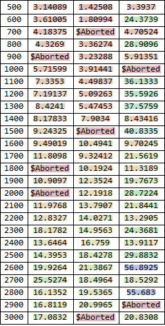
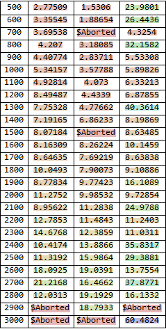
We see \$Aborted symbols at 1900,2300, and 2600 indicating these solutions greater that 30 seconds. On another machine, I let them solve to completion, but the problems occurred at 1900, 2600, and 2900 and were 2 orders of magnitude slower.

(*{
{"1500", "5.179350797570455`"},
{"1600", "5.721552865302039`"},
{"1700", "9.649557725880033`"},
{"1800", "7.249003463596244`"},
{"1900", "701.8212493274194`"},
{"2000", "9.54159604699469`"},
{"2100", "10.492328702172303`"},
{"2200", "15.721738736485552`"},
{"2300", "10.712554093479241`"},
{"2400", "12.832921044776027`"},
{"2500", "18.425538886796073`"},
{"2600", "1351.6927980656985`"},
{"2700", "25.303365975085192`"},
{"2800", "15.40859916429337`"},
{"2900", "1690.62244970152`"},
{"3000", "29.832779546846677`"}
}*)

We can compare the 1000 and 3000 case and see they look similar although the 1000 case is rougher at the beginning. It could be on the verge of instability.

alextelmod[10, 0.6, 1000][[4]]
alextelmod[10, 0.6, 3000][[4]]

enter image description here

enter image description here

To understand why certain MinPoints are unlucky will take more investigation. Robustness issues can be demoralizing. Perhaps the coupled approach would be more robust.

I hope this approach can help you isolate the problem.

Best regards,

Tim

Attachments:
POSTED BY: Tim Laska

Hi Markus,

I modified the module so that you could select from the three cases you provided plus I added some multiples of the original $\delta$ parameters and pass in some additional options.

<< DifferentialEquations`InterpolatingFunctionAnatomy`

solitonMod[tmx_, xmx_, minpt_, casename_, plottitle_] := 
 Module[{a, tmax, xmax, d3, d4, NS, Us1, eqs, bc, ic,
   time, sol, U2, UAbs, t1, t2,
   x1, x2, dp, plt, grid},
  (* d3=0.00404040404040404;
  d4=-4.2087542087542085*^-6;*)
  d3 := 0 /; casename == "Base";
  d4 := 0 /; casename == "Base";
  d3 := 0.00404040404040404 /; casename == "Orig";
  d4 := -4.2087542087542085*^-6 /; casename == "Orig";
  d3 := 5 0.00404040404040404 /; casename == "Orig5x";
  d4 := 5*(-4.2087542087542085*^-6) /; casename == "Orig5x";
  d3 := 2 0.00404040404040404 /; casename == "Orig2x";
  d4 := 2*(-4.2087542087542085*^-6) /; casename == "Orig2x";
  d3 := 2.5 0.00404040404040404 /; casename == "Orig2.5x";
  d4 := 2.5*(-4.2087542087542085*^-6) /; casename == "Orig2.5x";
  d3 := 3.0 0.00404040404040404 /; casename == "Orig3x";
  d4 := 3.0*(-4.2087542087542085*^-6) /; casename == "Orig3x";
  d3 := 0.04 /; casename == "0.04";
  d4 := 0 /; casename == "0.04";
  NS = 4;

  xmax = Rationalize[xmx];
  tmax = Rationalize[tmx];
  a = 1.3862943611198906;

  Us1[t_] = Exp[-a*t^2];
  Plot[Us1[t], {t, -tmax, tmax}, Frame -> True, 
   PlotStyle -> Darker[Blue], PlotRange -> All, Filling -> Bottom];
  eqs = {D[Us[t, x] , x] - I/2*D[Us[t, x], {t, 2}] - 
      d3*D[Us[t, x], {t, 3}]
      - I*d4*D[Us[t, x], {t, 4}] - I*NS^2*Abs[Us[t, x]]^2*Us[t, x] == 
     0}; 
       bc = {Us[tmax, x] == Us1[tmax], 
    Us[-tmax, x] == 
     Us1[-tmax], (D[Us[t, x], {t, 1}] /. 
       t -> tmax) == (D[Us1[t], {t, 1}] /. 
       t -> tmax), (D[Us[t, x], {t, 1}] /. 
       t -> -tmax) == (D[Us1[t], {t, 1}] /. t -> -tmax)};
      ic = {Us[t, 0] == Us1[t]};
  Print["seconds to obtain solution: ",
   time = AbsoluteTiming[
      Monitor[
        sol = 
         NDSolve[Join[eqs, ic, bc], 
          Us, {t, -tmax, tmax}, {x, 0, xmax}, 
          EvaluationMonitor :> (xcurrent = x), 
          Method -> {"MethodOfLines", 
            "SpatialDiscretization" -> {"TensorProductGrid", 
              "MinPoints" -> minpt, "DifferenceOrder" -> 8}}(*,
          PrecisionGoal\[Rule]5,AccuracyGoal\[Rule]5*), 
          MaxSteps -> 10000, (*MaxStepFraction -> 1/600*)], 
        "current x (\!\(\*SubscriptBox[\(x\), \(max\)]\)=" <> 
         ToString[xmax] <> "): " <> ToString[ xcurrent]];][[1]]] ;
  Print["grid points along {t,x}-directions: ", 
   Length /@ InterpolatingFunctionCoordinates[Us /. sol[[1]]]];
  U2[t_, x_] = Us[t, x] /. sol[[1]];
  UAbs[t_, x_] = U2[t, x] // Abs;
  t1 = -10.0; t2 = 10.0; x1 = 0.0; x2 = xmax;
  dp = 1;
  plt = 1;
  grid = 1;
  dp = DensityPlot[UAbs[t, x], {t, t1, t2}, {x, x1, x2}, 
    PerformanceGoal -> "Quality", ColorFunction -> "BlueGreenYellow", 
    PlotRange -> All, FrameLabel -> {"t=T/T0", "x=z/LD"}, 
    PlotLabel -> plottitle, MaxRecursion -> 4];
  plt = Plot3D[UAbs[t, x], {t, t1, t2}, {x, x1, x2}, 
    PerformanceGoal -> "Quality", ColorFunction -> "BlueGreenYellow", 
    PlotRange -> All, AxesLabel -> {"t=T/T0", "x=z/LD", "amplitude"}, 
    PlotLabel -> plottitle, MaxRecursion -> 5, ImageSize -> Large];
  grid = GraphicsRow[{dp, plt}, ImageSize -> 700];
  {time, sol, dp, plt, grid}
  ]
Options[solitonfn] = {"tmax" -> 10, "xmax" -> 0.6, 
   "minpoints" -> 2100, "case" -> "Base", 
   "title" -> "breathing of higher-order soliton"};
solitonfn[OptionsPattern[]] := 
 solitonMod[OptionValue["tmax"], OptionValue["xmax"], 
  OptionValue["minpoints"], OptionValue["case"], OptionValue["title"]]

I ran some cursory tests and I did not see much effect of accuracy and precision goals, so I commented them out. Then, I ran a more complete series varying the MinPoints option of your three cases on two machines and the timing results are shown below (note that I shutdown and restarted Mathematica and saw some shifts but over all about the same failure rates). The columns are the $\delta=0$, Original Parameters, and $\delta_3=0.04$, respectively.
enter image description here

enter image description here

The mesh adaptation process is going to be somewhat random and in my experience are slow. We see that there is little change going from low MinPoints to high MinPoints indicating insensitivity.
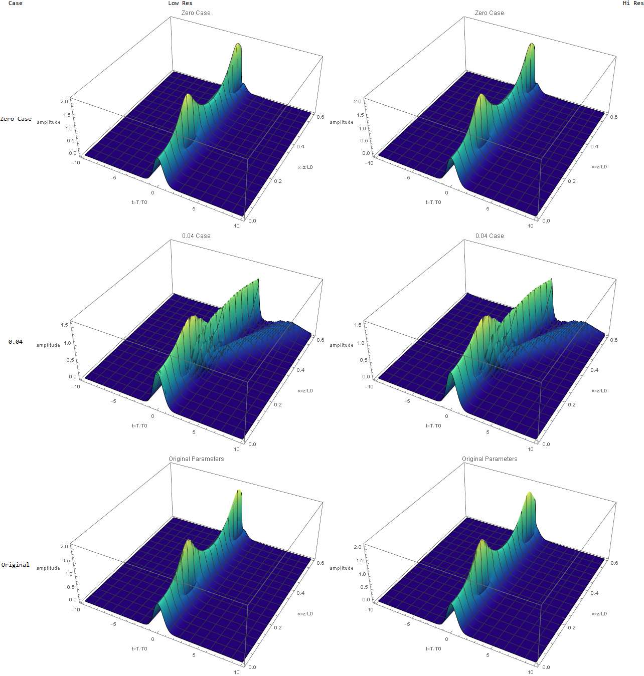
enter image description here

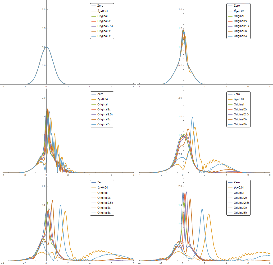
The original parameters seem to be stable and insensitive to MinPoints. Is there some some stability criterion for why they should be unstable? In any event, I ran a series to produce the animated gif below. At 2x the original parameters ( $\color{Red}{Red}$ curve), we start to see some ringing on the right tail. The ringing becomes more pronounced on the $\color{Purple}{Purple}$ curve at 2.5x original and you can see a fast moving shallow wave propagate to the right. At 3x, it is slower but higher amplitude.

hires0 = solitonfn["minpoints" -> 2800, "title" -> "Zero Case"];
hiresOrig = 
  solitonfn["case" -> "Orig", "minpoints" -> 2800, 
   "title" -> "Original Parameters"];
hiresOrig2x = 
  solitonfn["case" -> "Orig2x", "minpoints" -> 2900, 
   "title" -> "2x Original Parameters"];
hiresOrig25x = 
  solitonfn["case" -> "Orig2.5x", "minpoints" -> 2900, 
   "title" -> "2.5x Original Parameters"];
hiresOrig3x = 
  solitonfn["case" -> "Orig3x", "minpoints" -> 2900, 
   "title" -> "3x Original Parameters"];
hiresOrig5x = 
  solitonfn["case" -> "Orig5x", "minpoints" -> 2800, 
   "title" -> "5x Original Parameters"];
hires04 =  
  solitonfn["case" -> "0.04", "minpoints" -> 2800, 
   "title" -> "0.04 Case"];


f = ((#1 - #2)/(#3 - #2)) &;   
pltsComb = 
  Monitor[Table[
    Plot[{Evaluate[Abs[Us[\[Tau], i]] /. Last[hires0[[2]]]], 
      Evaluate[Abs[Us[\[Tau], i]] /. Last[hires04[[2]]]], 
      Evaluate[Abs[Us[\[Tau], i]] /. Last[hiresOrig[[2]]]], 
      Evaluate[Abs[Us[\[Tau], i]] /. Last[hiresOrig2x[[2]]]], 
      Evaluate[Abs[Us[\[Tau], i]] /. Last[hiresOrig25x[[2]]]], 
      Evaluate[Abs[Us[\[Tau], i]] /. Last[hiresOrig3x[[2]]]], 
      Evaluate[
       Abs[Us[\[Tau], i]] /. Last[hiresOrig5x[[2]]]]}, {\[Tau], -4, 
      8}, PlotRange -> {0, 2.25}, ImageSize -> Large, 
     PlotStyle -> Thick, 
     PlotLegends -> 
      Placed[LineLegend[{"Zero", 
         "\!\(\*SubscriptBox[\(\[Delta]\), \(3\)]\)=0.04", "Original",
          "Original2x", "Original2.5x", "Original3x", "Original5x"}, 
        LegendFunction -> Frame], {0.75, 0.75}]], {i, 0, 0.6, 0.003}],
    Grid[{{"Total progress:", 
      ProgressIndicator[
       Dynamic[f[i, 0, 0.6, 0.003]]]}, {"i=", {Dynamic@i}}}]];
enter image description here

The module seems to be behaving in consistent way and will solve in less than 10 seconds for many cases. At the current solver settings, the simulation hangs about 20% of the time in a random fashion. Now, the Test Analyze and Fix phase kicks in.

POSTED BY: Tim Laska

Hi Tim.

Thank you for all your effort. This is really the point, the adaptive meshing sometimes causes the simulations to go extremely slow. No idea how to address this. Do you have experience with that?

Could you send me the Notebooks as files? I tried to run your codes but it did not work.

Best,

Markus

POSTED BY: Markus Schmidt

Hi Markus,

There are many potential ways to deal with this issue. In an ideal world, you would provide robust simulation settings and it would solve in a predictable way. Generally, it can take 100s to 1000s of simulations to find optimal and robust simulation settings. Alternatively, you could try less glamorous approaches such as detection, preemption, and restarting the simulation. For example, you could use wrap the process in while loop and use the TimeConstrained function to stop crawling simulations and restart them with another MinPoints value. Of course, you don't want to stop a bunch of simulations that are about to finish, so you need a good balking time. While the process is autonomously running in the background at 80%, you can be investigating better approaches, but at least you are getting some work done.

The mesh is always adapting, it is just that it sometime gets confused. What would be ideal is if we could supply a pre-refined non-uniform mesh as an initial starting point like we do with the FEM technique. We would have a fine mesh in the center and coarser mesh in the wings. Then the solver as an initial guess for refinement. Solvers work best when supplied with good initial guesses. I don't think this is an option with the Numerical Method of Lines.

Also, I zoomed in to get a better look at the "fission". You might want take a look to verify that it is behaving physically.

enter image description here

Finally, I added $Sech^2$ option for a pulse. It should not underflow like the Gaussian at large absolute time. I tested it out on $x=1.8$ and $\tau_{max}=20$ for the original case. You can see some "fission" taking place where it did not appear to full develop in the shorter domain.

Short Domain

enter image description here

Bigger Domain

enter image description here

I hope that we are in better region than when we started.

Best regards,

Tim

POSTED BY: Tim Laska

Hi Tim.

Thank you very much for the idea of warping the solution into a loop and change MinPoints (and your code). I did that by placing the code into TimeConstrained (to terminate the calculation after a predefined time) and by checking if there is an accuracy warning after the simulation is finished (code is attached). The result is shown in this figure: - red points: simulations finish within 30s, but delivery insufficient accuracy.
- blue points: the simulation have been terminated after 30s - green points: simulations are good (<30s and sufficient accuracy) enter image description here As you see there exists somehow randomly distributed situations that the simulation time is very high, but slight variations of MinPoints lead to simulation time <30s. This plot clearly suggests that there is no systematic strategy to pick a good MinPoints, it needs to be tried out. However, for me this is not a problem since I can try a few MinPoints and then get some work done (as you correctly said). I simulated a slightly different problem and also found green points, so it is good. Thank you for all your suggestion, I was not aware of this problem. Markus

Attachments:
POSTED BY: Markus Schmidt

An error occurs when calculating the function Us1[\[Tau]]. The interval {\[Tau], -\[Tau]max, \[Tau]max} is selected too large. It is necessary to reduce the interval by an order of magnitude, to set the agreed boundary conditions and improve the accuracy of calculations, to choose the correct method. Then we have a solution to the equation

\[Delta]3 = 0.00404040404040404`30;
\[Delta]4 = -4.2087542087542085`30*^-6;
NS = 4.483404754211932`30;
NS2 = 20.100918190090154388694371172624`30;
\[Xi]max = 1;
\[Tau]max = 3;
q = 1.3862943611198906`30;
Us1[\[Tau]_] = Exp[-q*\[Tau]^2];
Plot[Us1[\[Tau]], {\[Tau], -\[Tau]max, \[Tau]max}, Frame -> True, 
 PlotStyle -> Darker[Blue], PlotRange -> All, Filling -> Bottom]
eqs = {D[Us[\[Tau], \[Xi]] , \[Xi]] - 
     I/2*D[Us[\[Tau], \[Xi]], {\[Tau], 2}] - \[Delta]3*
      D[Us[\[Tau], \[Xi]], {\[Tau], 3}] - 
     I*\[Delta]4*D[Us[\[Tau], \[Xi]], {\[Tau], 4}] - 
     I*NS2*Abs[Us[\[Tau], \[Xi]]]^2*Us[\[Tau], \[Xi]] == 0}; 
bc = {Us[\[Tau]max, \[Xi]] == Us1[\[Tau]max], 
   Us[-\[Tau]max, \[Xi]] == 
    Us1[-\[Tau]max], (D[
       Us[\[Tau], \[Xi]], {\[Tau], 1}] /. \[Tau] -> \[Tau]max) == (D[
       Us1[\[Tau]], {\[Tau], 1}] /. \[Tau] -> \[Tau]max), (D[
       Us[\[Tau], \[Xi]], {\[Tau], 1}] /. \[Tau] -> -\[Tau]max) == (D[
       Us1[\[Tau]], {\[Tau], 1}] /. \[Tau] -> -\[Tau]max)};
ic = {Us[\[Tau], 0] == Us1[\[Tau]]};


sol = NDSolve[Join[eqs, ic, bc], 
   Us, {\[Tau], -\[Tau]max, \[Tau]max}, {\[Xi], 0, \[Xi]max}, 
   Method -> {"MethodOfLines", 
     "SpatialDiscretization" -> {"TensorProductGrid", 
       "MinPoints" -> 40, "MaxPoints" -> 100, 
       "DifferenceOrder" -> "Pseudospectral"}}, MaxSteps -> 10^6, 
   WorkingPrecision -> 20] // AbsoluteTiming
Plot3D[Abs[Us[\[Tau], \[Xi]]] /. 
  Last[sol], {\[Tau], -\[Tau]max, \[Tau]max}, {\[Xi], 0, \[Xi]max}, 
 Mesh -> None, ColorFunction -> Hue, PlotRange -> All]

fig1

Your code takes very long time on my machine. The large time interval is required here, since the higher order solution undergoes fission due to the perturbation, leading to a slow linear wave.

POSTED BY: Markus Schmidt

I offered you a working code for solving your problem. You can change the parameters to calculate faster, for example, lower the accuracy of the calculations, setting "MaxPoints" -> 80`andWorkingPrecision -> 15`.

Posted 6 years ago

Hi Markus, I assume MaxStepSize if the maximum acceptable increment of your variable when walking through your solution space. Usually this size gets reduced automatically when the gradient increases in order to reduce the error. 80s sounds reasonable to me, I have done similar simulations for the propagation of wave packets according to Schrödinger's equation.

POSTED BY: Markus Lenzing

Thank you for the help. May I ask what kind of code you have used to solve the nonlinear Schroedinger equation? Did that include dispersion? May I see your code? Best, Markus

POSTED BY: Markus Schmidt
Reply to this discussion
Community posts can be styled and formatted using the Markdown syntax.
Reply Preview
Attachments
Remove
or Discard

Group Abstract Group Abstract