Hi Markus,
I modified the module so that you could select from the three cases you provided plus I added some multiples of the original
$\delta$ parameters and pass in some additional options.
<< DifferentialEquations`InterpolatingFunctionAnatomy`

solitonMod[tmx_, xmx_, minpt_, casename_, plottitle_] :=
 Module[{a, tmax, xmax, d3, d4, NS, Us1, eqs, bc, ic,
   time, sol, U2, UAbs, t1, t2,
   x1, x2, dp, plt, grid},
  (* d3=0.00404040404040404;
  d4=-4.2087542087542085*^-6;*)
  d3 := 0 /; casename == "Base";
  d4 := 0 /; casename == "Base";
  d3 := 0.00404040404040404 /; casename == "Orig";
  d4 := -4.2087542087542085*^-6 /; casename == "Orig";
  d3 := 5 0.00404040404040404 /; casename == "Orig5x";
  d4 := 5*(-4.2087542087542085*^-6) /; casename == "Orig5x";
  d3 := 2 0.00404040404040404 /; casename == "Orig2x";
  d4 := 2*(-4.2087542087542085*^-6) /; casename == "Orig2x";
  d3 := 2.5 0.00404040404040404 /; casename == "Orig2.5x";
  d4 := 2.5*(-4.2087542087542085*^-6) /; casename == "Orig2.5x";
  d3 := 3.0 0.00404040404040404 /; casename == "Orig3x";
  d4 := 3.0*(-4.2087542087542085*^-6) /; casename == "Orig3x";
  d3 := 0.04 /; casename == "0.04";
  d4 := 0 /; casename == "0.04";
  NS = 4;

  xmax = Rationalize[xmx];
  tmax = Rationalize[tmx];
  a = 1.3862943611198906;

  Us1[t_] = Exp[-a*t^2];
  Plot[Us1[t], {t, -tmax, tmax}, Frame -> True,
   PlotStyle -> Darker[Blue], PlotRange -> All, Filling -> Bottom];
  eqs = {D[Us[t, x] , x] - I/2*D[Us[t, x], {t, 2}] -
      d3*D[Us[t, x], {t, 3}]
      - I*d4*D[Us[t, x], {t, 4}] - I*NS^2*Abs[Us[t, x]]^2*Us[t, x] ==
     0};
       bc = {Us[tmax, x] == Us1[tmax],
    Us[-tmax, x] ==
     Us1[-tmax], (D[Us[t, x], {t, 1}] /.
       t -> tmax) == (D[Us1[t], {t, 1}] /.
       t -> tmax), (D[Us[t, x], {t, 1}] /.
       t -> -tmax) == (D[Us1[t], {t, 1}] /. t -> -tmax)};
      ic = {Us[t, 0] == Us1[t]};
  Print["seconds to obtain solution: ",
   time = AbsoluteTiming[
      Monitor[
        sol =
         NDSolve[Join[eqs, ic, bc],
          Us, {t, -tmax, tmax}, {x, 0, xmax},
          EvaluationMonitor :> (xcurrent = x),
          Method -> {"MethodOfLines",
            "SpatialDiscretization" -> {"TensorProductGrid",
              "MinPoints" -> minpt, "DifferenceOrder" -> 8}}(*,
          PrecisionGoal\[Rule]5,AccuracyGoal\[Rule]5*),
          MaxSteps -> 10000, (*MaxStepFraction -> 1/600*)],
        "current x (\!\(\*SubscriptBox[\(x\), \(max\)]\)=" <>
         ToString[xmax] <> "): " <> ToString[ xcurrent]];][[1]]] ;
  Print["grid points along {t,x}-directions: ",
   Length /@ InterpolatingFunctionCoordinates[Us /. sol[[1]]]];
  U2[t_, x_] = Us[t, x] /. sol[[1]];
  UAbs[t_, x_] = U2[t, x] // Abs;
  t1 = -10.0; t2 = 10.0; x1 = 0.0; x2 = xmax;
  dp = 1;
  plt = 1;
  grid = 1;
  dp = DensityPlot[UAbs[t, x], {t, t1, t2}, {x, x1, x2},
    PerformanceGoal -> "Quality", ColorFunction -> "BlueGreenYellow",
    PlotRange -> All, FrameLabel -> {"t=T/T0", "x=z/LD"},
    PlotLabel -> plottitle, MaxRecursion -> 4];
  plt = Plot3D[UAbs[t, x], {t, t1, t2}, {x, x1, x2},
    PerformanceGoal -> "Quality", ColorFunction -> "BlueGreenYellow",
    PlotRange -> All, AxesLabel -> {"t=T/T0", "x=z/LD", "amplitude"},
    PlotLabel -> plottitle, MaxRecursion -> 5, ImageSize -> Large];
  grid = GraphicsRow[{dp, plt}, ImageSize -> 700];
  {time, sol, dp, plt, grid}
  ]
Options[solitonfn] = {"tmax" -> 10, "xmax" -> 0.6,
   "minpoints" -> 2100, "case" -> "Base",
   "title" -> "breathing of higher-order soliton"};
solitonfn[OptionsPattern[]] :=
 solitonMod[OptionValue["tmax"], OptionValue["xmax"],
  OptionValue["minpoints"], OptionValue["case"], OptionValue["title"]]
I ran some cursory tests and I did not see much effect of accuracy and precision goals, so I commented them out. Then, I ran a more complete series varying the MinPoints option of your three cases on two machines and the timing results are shown below (note that I shutdown and restarted Mathematica and saw some shifts but over all about the same failure rates). The columns are the
$\delta=0$, Original Parameters, and
$\delta_3=0.04$, respectively.
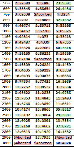
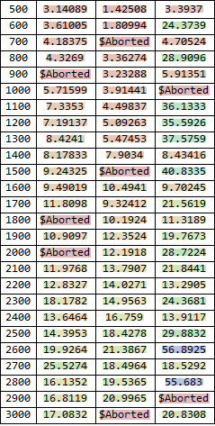
The mesh adaptation process is going to be somewhat random and in my experience are slow.
We see that there is little change going from low MinPoints to high MinPoints indicating insensitivity.
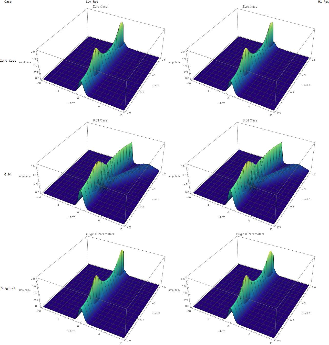
The original parameters seem to be stable and insensitive to MinPoints. Is there some some stability criterion for why they should be unstable? In any event, I ran a series to produce the animated gif below. At 2x the original parameters (
$\color{Red}{Red}$ curve), we start to see some ringing on the right tail. The ringing becomes more pronounced on the
$\color{Purple}{Purple}$ curve at 2.5x original and you can see a fast moving shallow wave propagate to the right. At 3x, it is slower but higher amplitude.
hires0 = solitonfn["minpoints" -> 2800, "title" -> "Zero Case"];
hiresOrig =
  solitonfn["case" -> "Orig", "minpoints" -> 2800,
   "title" -> "Original Parameters"];
hiresOrig2x =
  solitonfn["case" -> "Orig2x", "minpoints" -> 2900,
   "title" -> "2x Original Parameters"];
hiresOrig25x =
  solitonfn["case" -> "Orig2.5x", "minpoints" -> 2900,
   "title" -> "2.5x Original Parameters"];
hiresOrig3x =
  solitonfn["case" -> "Orig3x", "minpoints" -> 2900,
   "title" -> "3x Original Parameters"];
hiresOrig5x =
  solitonfn["case" -> "Orig5x", "minpoints" -> 2800,
   "title" -> "5x Original Parameters"];
hires04 =
  solitonfn["case" -> "0.04", "minpoints" -> 2800,
   "title" -> "0.04 Case"];


f = ((#1 - #2)/(#3 - #2)) &;
pltsComb =
  Monitor[Table[
    Plot[{Evaluate[Abs[Us[\[Tau], i]] /. Last[hires0[[2]]]],
      Evaluate[Abs[Us[\[Tau], i]] /. Last[hires04[[2]]]],
      Evaluate[Abs[Us[\[Tau], i]] /. Last[hiresOrig[[2]]]],
      Evaluate[Abs[Us[\[Tau], i]] /. Last[hiresOrig2x[[2]]]],
      Evaluate[Abs[Us[\[Tau], i]] /. Last[hiresOrig25x[[2]]]],
      Evaluate[Abs[Us[\[Tau], i]] /. Last[hiresOrig3x[[2]]]],
      Evaluate[
       Abs[Us[\[Tau], i]] /. Last[hiresOrig5x[[2]]]]}, {\[Tau], -4,
      8}, PlotRange -> {0, 2.25}, ImageSize -> Large,
     PlotStyle -> Thick,
     PlotLegends ->
      Placed[LineLegend[{"Zero",
         "\!\(\*SubscriptBox[\(\[Delta]\), \(3\)]\)=0.04", "Original",
          "Original2x", "Original2.5x", "Original3x", "Original5x"},
        LegendFunction -> Frame], {0.75, 0.75}]], {i, 0, 0.6, 0.003}],
    Grid[{{"Total progress:",
      ProgressIndicator[
       Dynamic[f[i, 0, 0.6, 0.003]]]}, {"i=", {Dynamic@i}}}]];
The module seems to be behaving in consistent way and will solve in less than 10 seconds for many cases. At the current solver settings, the simulation hangs about 20% of the time in a random fashion. Now, the Test Analyze and Fix phase kicks in.


