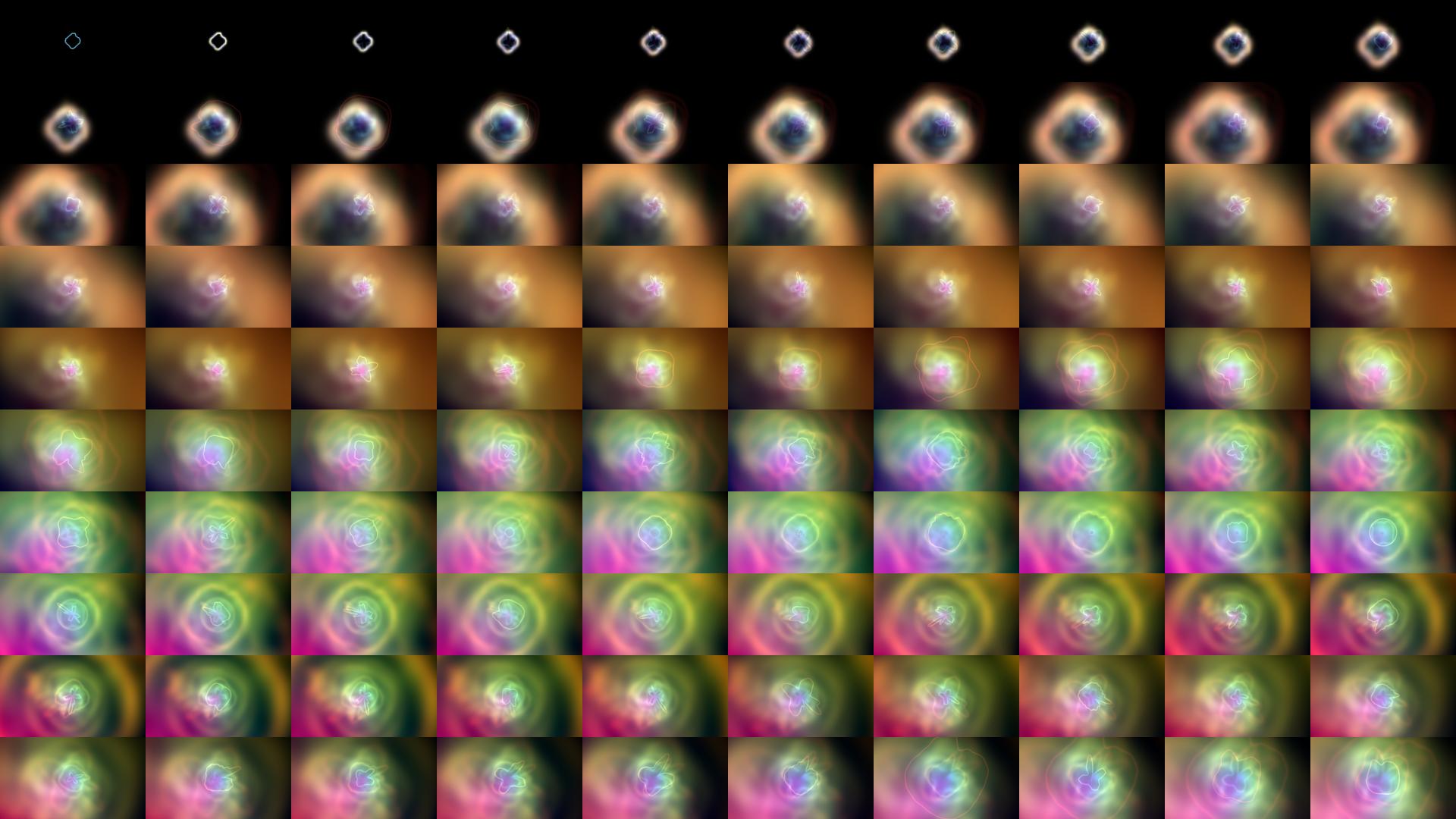
Click image to zoom in. Use browser back button to read further.

Over the Christmas holidays, I finally found some time to test out something I had in mind for a while: Creating an abstract visualization of music. These things are well known and are built into many music-players, but I never tried it myself. If you want to know the whole story behind it you can read my blog-post about home-recording.

What I did is importing an MP3 into Mathematica and using AudioLocalMeasurements to extract frequencies and loudness of the song.

audio = Import[file];
meas = AudioLocalMeasurements[audio, {"MFCC", "Loudness"}, 
         Association, PartitionGranularity -> Quantity[1./30., "Seconds"]];

This gives two TimeSeries and lets you extract values for every time point of the song. The MFCC is a list of numbers that represent (afaik) the strengths of certain frequencies. The loudness is a single number and gives an estimated loudness measure of the portion.

To visualize it, I used a single ParametricPlot that uses the frequency-strengths as factors of a simple trigonometric sum which is plotted in a circular fashion. The size of the circular structure is influenced by the loudness and in addition, it rotates slowly over time. To colorize the plot, I used the distance from the origin and employed one of Mathematica’s color schemes. The majority of the function below is setting-up options to create a plot with fixed plot-range, aspect ratio, etc., and turn it into a slightly blurred image of fixed resolution.

(* Change the line below if you want full HD *)
resolution = {1920, 1080}/10;
ratio = Divide @@ resolution;

With[{mfcc = meas["MFCC"], loudness = Rescale[meas["Loudness"]]},
 gr[time_?NumericQ] := With[{f = mfcc[time], l = loudness[time]},
   Block[{img, t},
    With[{s = Sum[4 f[[i]]*Sin[(i + 3)*t], {i, Length[f]}]},
     img = 
      ParametricPlot[(s + 2 l + .1) {Cos[t + .2 time], Sin[t + .2 time]}, {t, 0, 2 Pi},
       PlotRange -> {{-2, 2}*ratio, {-2, 2}},
       PlotRangeClipping -> True,
       PlotRangePadding -> None,
       PlotStyle -> Directive[Thickness[0.008]],
       Axes -> False, 
       ColorFunction -> Function[{x, y, u}, ColorData["Rainbow", Norm[{x, y}]]],
       ColorFunctionScaling -> False,
       Background -> Black,
       AspectRatio -> 1/ratio];
     GaussianFilter[Rasterize[img, ImageSize -> resolution], First[resolution]/400.]
     ]]
   ]
 ]

 gr[250]

This is how a frame at t=250s looks like

Unspectacular to say the least, but we are not quite done. A simple trick to make it more interesting is to Fold frames so that the old frame leaves a trace in each subsequent image. Specifically, I blurred the old frame, enlarged it and cropped it back to the original size. It is then added to the current frame, where I give the old frame a higher weight before using ImageAdjust to rescale all pixel values. This makes everything very colorful and foggy, and the enlargement gives the impression as if we would move forward in space.

tstart = 100;
FoldList[
  ImageAdjust[
    ImageCrop[
      ImageResize[5 GaussianFilter[#1, First[resolution]/100.], Scaled[22/20]],
      resolution
    ] + gr[#2]
  ] &,   
  gr[tstart], Range[tstart, tstart + 100]
]

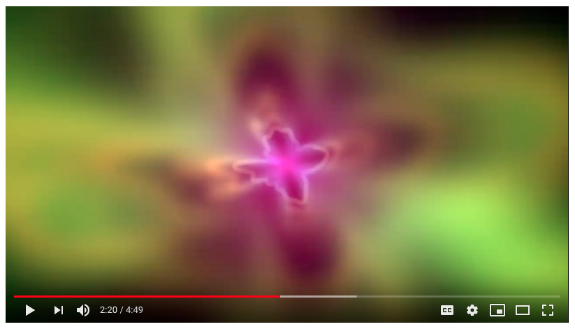
The above is now used to create a frame each 1/30th second which is then exported as an image. After all frames are created, I merged the music and the single frames into one video using ffmpeg, and I have outlined more details on my webpage. Here is video of the final result and I hope you like it.