The webcomic xkcd featured an interesting comic for March 1, 2019:

Rarely would I be accused of taking a joke (too) seriously, but I found this intriguing enough to try doing this in Mathematica.

That is, what should the lower and upper limits be such that the vertical area is equal to $\frac12$ (recalling that the area under a PDF should be $1$)?

Let's first define the PDF of the normal distribution (i.e. the usual bell curve):

pdf[x_] = PDF[NormalDistribution[], x]
   E^(-(x^2/2))/Sqrt[2 ?]

As in the comic, I will make the arbitrary and capricious choice of centering the area of interest at

pdf[0]/2
   1/(2 Sqrt[2 ?])

One thing to do is to find the abscissas corresponding to the upper and lower limits; that is, if we let the height of the area be 2 h, find the value of x such that pdf[x] == 1/(2 Sqrt[2 ?]) - h for the lower limit, and the value of x such that pdf[x] == 1/(2 Sqrt[2 ?]) + h for the upper limit. Due to the symmetry of the Gaussian function, it suffices to give the restriction x > 0:

{xm[h_], xp[h_]} = Assuming[-(1/(2 Sqrt[2 ?])) < h < 1/(2 Sqrt[2 ?]), 
                            Simplify[(x /. First[Solve[pdf[x] == 1/(2 Sqrt[2 ?]) + #
                                                       && x > 0, x]]) & /@ {-h, h}]]
   {Sqrt[2] Sqrt[-Log[1/2 - h Sqrt[2 ?]]], Sqrt[2] Sqrt[-Log[1/2 + h Sqrt[2 ?]]]}

where I have taken the liberty to assign the results to functions for later use.

At this point, one might wish to construct a Manipulate[] object to assist visualization, like so:

Manipulate[Plot[{Min[pdf[x], 1/(2 Sqrt[2 ?]) - h], 
                 Min[pdf[x], 1/(2 Sqrt[2 ?]) + h], pdf[x]}, {x, -4, 4}, 
                Exclusions -> None, Filling -> {2 -> {{1}, Opacity[0.6, Pink]}}, 
                PlotLabel -> StringForm["h=`1`, Area=`2`", h, 
                                        Quiet[2 NIntegrate[
                                              Min[pdf[x], 1/(2 Sqrt[2 ?]) + h] - 
                                              Min[pdf[x], 1/(2 Sqrt[2 ?]) - h],
                                              {x, 0, xm[h]}]]], 
                PlotStyle -> {None, None, ColorData[97, 1]}],
            {h, 0, 1/(2 Sqrt[2 ?])}]

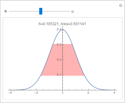
where I used Min[] to clip the Gaussian function at appropriate limits.

Note that in the example I gave, a value of $h\approx 0.105$ gives an area that is nearly equal to $\frac12$. To solve for the right value of $h$, let us get an explicit expression for the integral:

area = Assuming[0 < h < 1/(2 Sqrt[2 ?]), 
                Simplify[Integrate[Min[pdf[x], 1/(2 Sqrt[2 ?]) + h] - 
                                   Min[pdf[x], 1/(2 Sqrt[2 ?]) - h],
                                   {x, -xm[h], xm[h]}]]]

which yields a complicated expression involving the error function Erf[]. This can now be plugged into Solve[]:

hs = h /. First[Solve[area == 1/2 && 0 < h < 1/(2 Sqrt[2 ?]), h]];

which yields a complicated Root[] object that nevertheless can be easily evaluated numerically:

N[hs, 20]
   0.10508624993771281943

We also find that

2 hs/(pdf[0]) 100 // N
   52.6824

that is, the height of the area being considered covers $\approx 52.7\%$ of the whole height of the bell curve.

Let's show a hopefully more understandable way to solve for $h$. The area of interest can also be determined through a sequence of subtractions, which can be depicted pictorially:

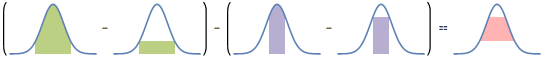
To do this, we need the expression for the area under a symmetric portion of the bell curve:

Assuming[a > 0, Integrate[pdf[x], {x, -a, a}]]
   Erf[a/Sqrt[2]]

Then, the necessary area expression is

area2 = (Erf[xm[h]/Sqrt[2]] - (2 xm[h]) (1/(2 Sqrt[2 ?]) - h)) -
        (Erf[xp[h]/Sqrt[2]] - (2 xp[h]) (1/(2 Sqrt[2 ?]) + h));

from which one can solve for the necessary value of $h$:

h /. First[Solve[area2 == 1/2 && 0 < h < 1/(2 Sqrt[2 ?]), h]]

which should again yield the same Root[] expression.