The following demonstration shows the use of Discrete Variable Representation to estimate the eigenstates of a quartic potential.

This demonstration is inspired by a homework problem in MIT Chemistry's graduate first-semester quantum mechanics class (5.73), as taught by Bob Field in Fall 2018. The problem was to find the first 106 eigenstates of the potential $v(x)=\frac{10^4x^2}{2} -1980 x^2 +200 x^4 $ , because there were 53 bound states (by the WKB quantization condition).

The approach, given by John Light and explained and applied in Harris, et al (1965), is as follows:

I) Take the x operator matrix in the harmonic oscillator basis, given by $$ \mathbf x = (\frac{\hbar}{2 m \omega})^{1/2} \begin{bmatrix} 0 & \sqrt{1} & 0 & 0 & \cdots \\ \sqrt{1} & 0 & \sqrt{2} & 0 & \cdots \\ 0 & \sqrt{2} & 0 & \sqrt{3} & \cdots \\ 0 & 0 & \sqrt{3} & 0 & \cdots \\ \vdots & \vdots & \vdots & \vdots & \ddots \end{bmatrix} $$ ...and diagonalize the $\mathbf x$ matrix by a similarity transformation such that $\lambda = T^{-1} \mathbf{x} T$.

II) Apply the potential function to the diagonal elements of $\lambda$ to compute $V(\lambda)$.

III) Transform $V(\lambda)$ back to the original representation, i.e. compute $V(x) = T V(\lambda) T^{-1}$.

IV) Compose the Hamiltonian matrix in the usual way by $H=\frac{p^2}{2 m}+V(x)$, expressing $p^2$ in the harmonic oscillator basis, and diagonalize this matrix.

Building it up

For purposes of this problem, let:

hbar=1
m = 1.000*10^-2
k = 1.000*10^4
omega = Sqrt[k/m]

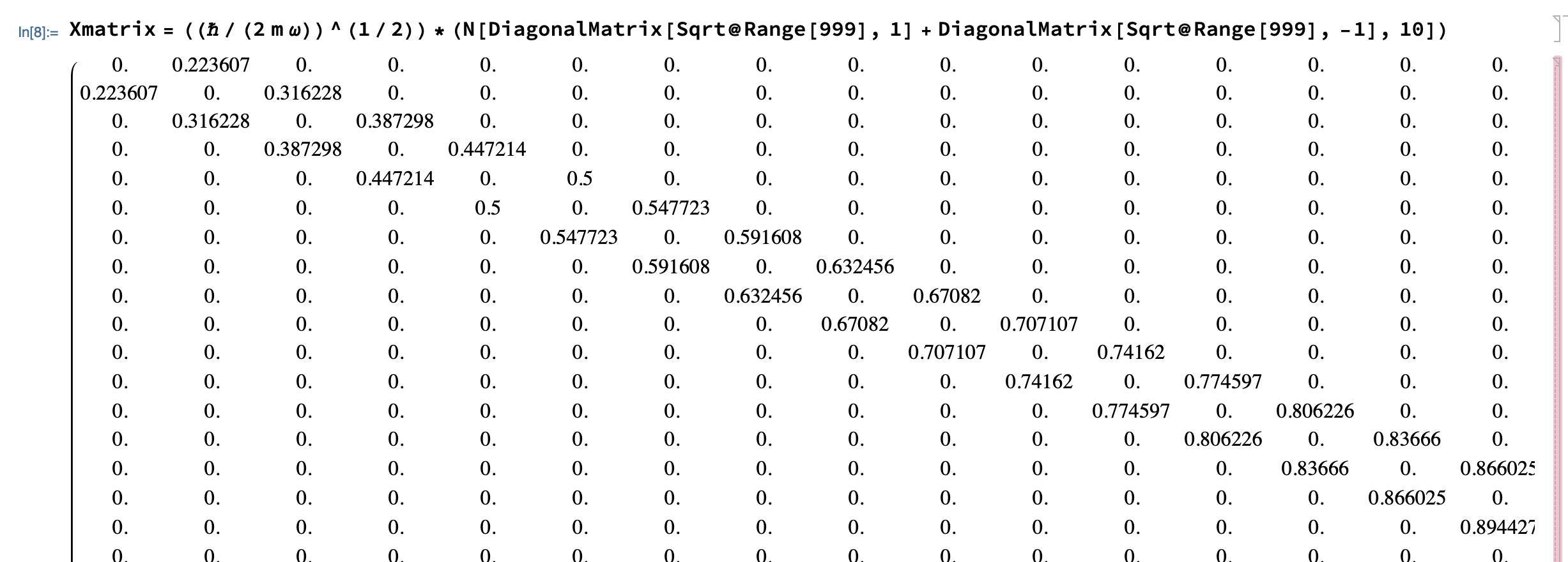
The x matrix in the harmonic oscillator basis can be defined as follows:

Xmatrix = 
 N[((hbar/(2 m omega))^(1/2))*(DiagonalMatrix[Sqrt@Range[999], 
      1] + DiagonalMatrix[Sqrt@Range[999], -1])] 

Then we diagonalize the X matrix:

{Xeivals, Xeivecs} = Eigensystem[Xmatrix]

The first few eigenvalues should be {13.9802, -13.9802, -13.856, 13.856, -13.7543}. The output can be checked by a classic eigenvalue test. Extremely small matrix elements will differ.

Xmatrix.Xeivecs[[1]]
Xeivecs[[1]]*Xeivals[[1]]

To associate eigenvalue-eigenvector pairs:

Xeigensystemtogether = AssociationThread[Xeivals -> Xeivecs]

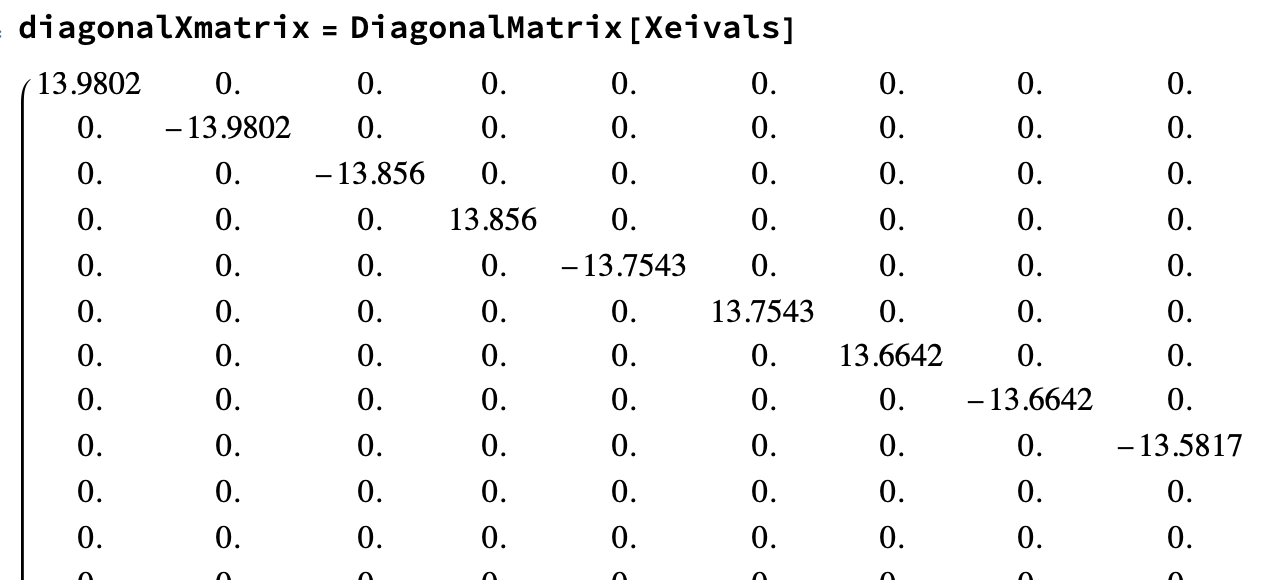
Now to define the $\lambda$ matrix, one can just use the DiagonalMatrix[] function specifying that the x eigenvalues are on the diagonal:

diagonalXmatrix = DiagonalMatrix[Xeivals]

To define the $V(\lambda)$ matrix:

Vlambdamatrix = DiagonalMatrix[vinput[Xeivals]]

Now, the diagonalizing transformation matrix T is by definition the matrix of the eigenvectors. Eigenvectors are returned as lists of row vectors in Mathematica, but mathematically we need them to be columns:

Tmatrix = Transpose[Xeivecs]

Since T is unitary, $T^{-1} = T^\dagger$...

Tdaggermatrix = ConjugateTranspose[Tmatrix]

Now to use $V(x) = T V(\lambda) T^{-1}$ to transform the V matrix back to the Harmonic Oscillator basis.

Vx = Tmatrix.Vlambdamatrix.Tdaggermatrix

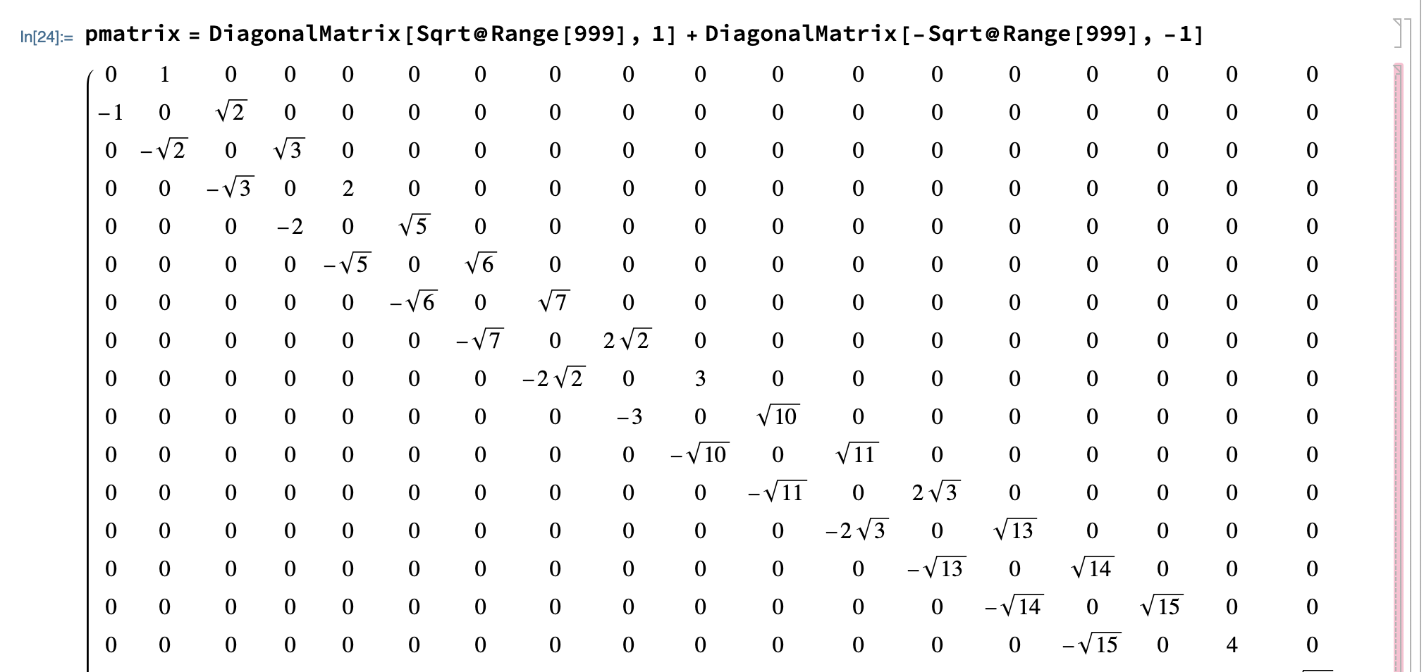
Defining a p matrix in the Harmonic Oscillator basis without the constants:

pmatrix = 
 DiagonalMatrix[Sqrt@Range[999], 1] + 
  DiagonalMatrix[-Sqrt@Range[999], -1]

The $p^2$ matrix:

psquared = N[((-hbar m omega)/2)*(pmatrix.pmatrix)]

Now to apply $H=\frac{p^2}{2 m} +V(x)$

Hmatrix = ((1/(2 m))*psquared) + Vx

And take the eigenvalues:

{Heivals, Heivecs} = Eigensystem[Hmatrix]

And the first (largest) few eigenvalues in this case are: ${1.40344*10^7, 1.36124*10^7, 1.32736*10^7, 1.29792*10^7, 1.27142*10^7, 1.24706*10^7,...}$.

Again for convenience, associating eigenvalue-eigenvector pairs and sorting smallest to largest:

Heigentogether = AssociationThread[Heivals -> Heivecs]
Heigensorted = KeySort[Heigentogether]

To extract the eigenvalues then the eigenvectors:

Hvalssorted = Keys[Heigensorted]
Hvecssorted = Values[Heigensorted]

The actual answer to the question:

Hvalssorted[[1 ;; 106]]

The first few are: 496.041, 1471.67, 2421.24, 2851.1, 3342.48, 3758.34

Combining into one function

To run DVR in the harmonic oscillator basis in three lines of code, define the potential function:

vinput[x_] = (10^4/2) x^2 - 1980 x^3 + 200 x^4

Then define the following module function, where expr_ is the name of the potential function and n_ is the dimension of matrices desired:

DVR[expr_, hbar_, m_, k_, n_] := 
 Module[{omega, x, xeivals, xeivecs, Vlambda, T, Tinv, Vx, p, 
   psquared, H, Heivals, Heivecs},
  omega = Sqrt[k/m];
  x = ((hbar/(2 m omega))^(1/2))*(N[
      DiagonalMatrix[Sqrt@Range[n - 1], 1] + 
       DiagonalMatrix[Sqrt@Range[n - 1], -1]]);
  {xeivals, xeivecs} = Eigensystem[x];
  Vlambda = DiagonalMatrix[expr[xeivals]];
  T = Transpose[xeivecs];
  Tinv = ConjugateTranspose[T];
  Vx = T.Vlambda.Tinv;
  p = N[DiagonalMatrix[Sqrt@Range[n - 1], 1] + 
     DiagonalMatrix[-Sqrt@Range[n - 1], -1]];
  psquared = N[((-hbar m omega)/2)*(p.p)];
  H = ((1/(2 m))*psquared) + Vx;
  {Heivals, Heivecs} = Eigensystem[H];
  {Heivals, Heivecs}]

To apply it to this problem:

{Heivalstest, Heivecstest} = DVR[vinput, 1, 0.01, 10000, 1000]

To test that the correct and needed eigenvalues are being output:

Part[Reverse@Heivalstest, 1 ;; 106]

Again, the first few values: 496.041, 1471.67, 2421.24, 2851.1, 3342.48, 3758.34.

Harris, David O., et al. "Calculation of Matrix Elements for One-Dimensional Quantum-MechanicalProblems and the Application toAnharmonic Oscillators." J. Chem. Phys. 43, 1515 (1965).