This revised code still has some issues.
Definition of the function f
- Although
x is one of the arguments, it is never used in the actual body of the definition, so why include it?
- The body of the definition is utterly too complicated, and there is no need whatsoever to use a
Module. or a separate variable dy.(And the definition, as given, is problemmatic: since dy is made global because it is not declared as a local variable to Module.)
- There is no need to include the vector dimension
m as an argument to f; let Mathematica determine it if it's needed.
The whole thing boils down to:
f[x_, yVec_] := {yVec[[2]], 6 yVec[[1]] - yVec[[2]]}
The definition of RK4
- I see utterly no need for giving
k1, k2, k3, k4 values as constant arrays in their declarations; they will become lists of length m automatically when you assign them values in the main body of the definition.
- Likewise, I see no need for the initialization step
yn1 = ConstantArray[0., m], because you directly assign a list of length m to yn1 as the last step.
- In fact, there's no need to do that: you don't need any
yn1 at all.
- There is no need to pass the vector dimension
m in as an argument!
- There are unnecessary uses of approximate numbers (i.e., numbers with decimals), provided that you have at least one such number involved in each computation. The simplest and cleanest way to do that is to take the numerical value, with
N, of the step size and use that afterwards.
- The separators
(* *) you include between lines seem utterly unnecessary and are, in fact, a bit distracting. (If you absolutely need to insert space between code lines, just use a blank line!)
Thus:
fixedRK4[x_, yn_, stepSize_] := Module[
  {k1 = k2 = k3 = k4, h = N[stepSize]},
  k1 = h f[x, yn];
  k2 = h f[x + h/2, yn + k1/2];
  k3 = h f[x + h/2, yn + k2/2];
  k4 = h f[x + h, yn + k3];
  yn+ 1/6 (k1 + 2 k2 + 2 k3 + k4)
  ]
The iteration: from explicit loop to implicit iteration
The next thing that needs work is that explicit loop. One way is to somewhat redesign RK4 so that it uses as its argument a list of the items you currently have as arguments and returns as output not just the list {x, y} of new values, but includes also m and h, as in the following. (I've renamed the function RK4step to indicate it carries out just one step of the Runge-Kutta process).
RK4step[{x_, y_, stepSize_}] := Module[
  {k1, k2, k3, k4, h = N[stepSize]},
  k1 = h f[x, y];
  k2 = h f[x + h/2, y + k1/2];
  k3 = h f[x + h/2, y + k2/2];
  k4 = h f[x + h, y + k3];
  {x + h, y + 1/6 (k1 + 2 k2 + 2 k3 + k4), h}
  ]
For example:
    RK4step[{0, {3., 1.}, 2, 0.1}]
(*  {0.1, {3.18364, 2.66309}, 0.1}  *)
The advantage of this modification is that it now allows you to feed the output from RK4step directly into a new call of RK4step. And this means that you may now use built-in "functional" operators of Mathematica to do the iteration for you automatically, using, say, NestList. (This will give much briefer, readable code and relegationg all details of performing iteration to Mathematica; doing this creates code that is not only briefer but also more efficient than coding the loop explicitly.) Thus:
NestList[RK4step, {0, {3., 1.}, 0.1}, 10]
In fact, we may now define a new function newRK4 that carries out this NestList for a user-specified number of steps. And give it as an argument not the number of steps, but the desired end value of x (your b) and the step-size, computing the corresponding number of steps inside newRK4:
newRK4[x0_, y0_, m_, xEnd_, stepSize_] :=
    Module[{n = Round[(xEnd - x0)/stepSize]},
         NestList[RK4step, {x0, y0, m, stepSize}, n]
    ]
(Alternatively, use the number of steps as the last argument and compute the corresponding step-size inside the function.)
Use it like this (I'll assign the output to a variable lis, to allow for further processing later):
lis = newRK4[0, {3., 1.}, 1, 0.1]
The output from that input is a long list of lists. The first two of those constituent lists will be:
{0, {3., 1.}, 0.1}
and
{0.1, {3.18364, 2.66309}, 0.1}
You now probably want to clean up the output in two ways:
1.Drop the step-size 0.1 from the end of each constituent list.
- Remove the innermost list braces in the
{x, y} 2nd entry of each constituent list.
To do 1: For a single list like {0, {3., 1.}, 0.1}, do this:
        Most[{0, {3., 1.}, 0.1}]
    (* {0, {3., 1.}} *)
To do all such dropping at once, use Map (shortcut abbreviation /@) of the function Most:
    shortlis = Most /@ lis
(* {{0, {3., 1.}}, {0.1, {3.18364, 2.66309}}, {0.2, {3.53248,
   4.32075}}, {0.3, {4.05081, 6.06862}}, {0.4, {4.75227,
   7.99841}}, {0.5, {5.65966, 10.2035}}, {0.6, {6.80547,
   12.7843}}, {0.7, {8.23275, 15.8531}}, {0.8, {9.99662,
   19.5396}}, {0.9, {12.1663, 23.9964}}, {1., {14.8276, 29.4062}}}*)
To do 2: To get rid of the innermost list braces in a single list such as {0, {3., 1.}} and convert it to {0, 3., 1._, use Flatten:
    Flatten[{0, {3., 1.}}]
(* {0, 3., 1.} *)
To do all such flattening at once, again use Map of the function Flatten:
nicelis = Flatten /@ shortlis
Combine refinements 1. and 2.:
nicelis = Flatten/@ Most /@ lis
In fact, we might as well take care of this dropping and flattening as part of the final RK4 function:
Putting this all together, we have:
        nicelis = Flatten/@ Most /@ newRK4[0, {3., 1.}, 1, 0.1]
    (*  {{0, 3., 1.}, {0.1, 3.18364, 2.66309}, {0.2, 3.53248, 4.32075}, {0.3,
      4.05081, 6.06862}, {0.4, 4.75227, 7.99841}, {0.5, 5.65966,
      10.2035}, {0.6, 6.80547, 12.7843}, {0.7, 8.23275, 15.8531}, {0.8,
      9.99662, 19.5396}, {0.9, 12.1663, 23.9964}, {1., 14.8276, 29.4062}}  *)
In fact, we might as well incorporate into a function RK4 that includes the flattening and most-ing:
nicerRK4[x0_, y0_, xEnd_, stepSize_] :=
 Flatten /@ Most /@ newRK4[x0, y0, xEnd, stepSize]
Now combine this nicerRK4 with the earlier newRK4 to form a single function RK4 that calls only RK4step and your f:
RK4[x0_, y0_, xEnd_, stepSize_] :=
 Module[{n = Round[(xEnd - x0)/stepSize]},
  Flatten /@ Most /@ NestList[RK4step, {x0, y0, stepSize}, n]]
Printing a nice table of results
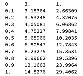
To get a nice looking table as output, use TableForm on the output from this RK4:
TableForm[RK4[0, {3., 1.}, 1, 0.1]]
The result look like this (no Print statements needed!)
If you want row or column headings, you can include those by using the TableHeadings option of TableForm or else by first prepending to nicelis a row of column heads and a column of row heads and then using Grid on the result. (Grid allows much fancier format control than does TableForm.)
Further refinements
Dependence on the function f: The function RK4step uses a function f that is defined globally. You could — and perhaps should — make f another argument of Rk4step, and then do the corresponding thing in RK4.
Input checking: For example, use:
    RK4[x0_NumericQ, y0_ (VectorQ || NumericQ), xEnd_NumericQ,
      stepSize_NumericQ] :=
     Module[{n = Round[(xEnd - x0)/stepSize]},
      Flatten /@ Most /@ NestList[RK4step, {x0, y0, stepSize}, n]]
Notice the condition (VectorQ || NumericQ) qualifying input y0. This is to allow use of RK4 either for a vector-valued user function f or a simple scalar-valued f. (The body of RK4 doesn't care which it is: the computations will proceed just fine in either case; that's part of the beauty of the design of the definition. To be sure, the flattening is not needed in the case of a scalar function, since each item in the overall list is already flat, but it will be harmless when included.)
Final comment
Why is the independent variable named x? More often than not, an ODE is a description of how a system behaves with respect to time. So it seems more natural to call the independent variable t rather than x.


