Introduction
Every day, millions of articles and posts are published on the web, spanning from sports to politics to science. But what would happen if AI systems became better than humans, learning from the huge amount of data and obtaining very high performance across many different tasks, using neural models and deep learning techniques based on Natural Language Processing (NLP)? In this post we will discuss a natural language processing topic, as much exciting as controversial, that uses deep learning techniques to summarize text: the GPT-2 model, one of the latest example of a new class of text-generation algorithms based on a transformer network trained with approximately more than 35 GB of text.
Summary
This project is designed for developing a text summarizer using Wolfram Mathematica software. Data preparation is an important and critical step in neural network data. We simplified the learning problem by adopting two different approaches: the first is about words with a given average length; the second one consists in splitting the body into paragraphs and create an association between the paragraphs and the highlights. To construct an embedding to capture the similarity of the words, we have used the pre-trained net Global Vectors (GloVe), stored in the neural net repositories on the Wolfram website (link: https://resources.wolframcloud.com/NeuralNetRepository/. Then, we trained the GPT-2 model, following the URL: https://openai.com/blog/better-language-models/. GPT-2 can predict a summary from the text, learning to generate text by studying a huge amount of data from the web and/or other sources. The GPT-2 is based on the Transformer, which is an attention model: it learns to focus attention to the previous token that is most relevant to the task requires: i.e., predicting the next word in a sentence generating a summary.
Data Exploration
In this project we are going to work with the CNN dataset. You can download the ASCII text of the stories at the following links: https://cs.nyu.edu/~kcho/DMQA/. The dataset was presented in the paper "Teaching Machines to Read and Comprehend" (2015) and it has been used in text summarization, in which sentences from the news articles are summarized. The dataset contains more than 92000 news articles. Each article is stored in a single .story file, that includes information on layout, styles used, images, formatting, fonts, etc. Another useful link on how to use some other packages to analyze the dataset is https://github.com/abisee/cnn-dailymail . We downloaded this dataset and unzipped it. Once unzipped the dataset, we imported it using the Import [] function , which returns a Wolfram Language representation of it, mapping (/@) the function FileName[], which lists all files in the current working directory, onto each individual element in the list.
data=Import[#,"Text"]&/@FileNames["/Users/sadinov/Desktop/TS/Datasets/cnn/stories/*.story"];
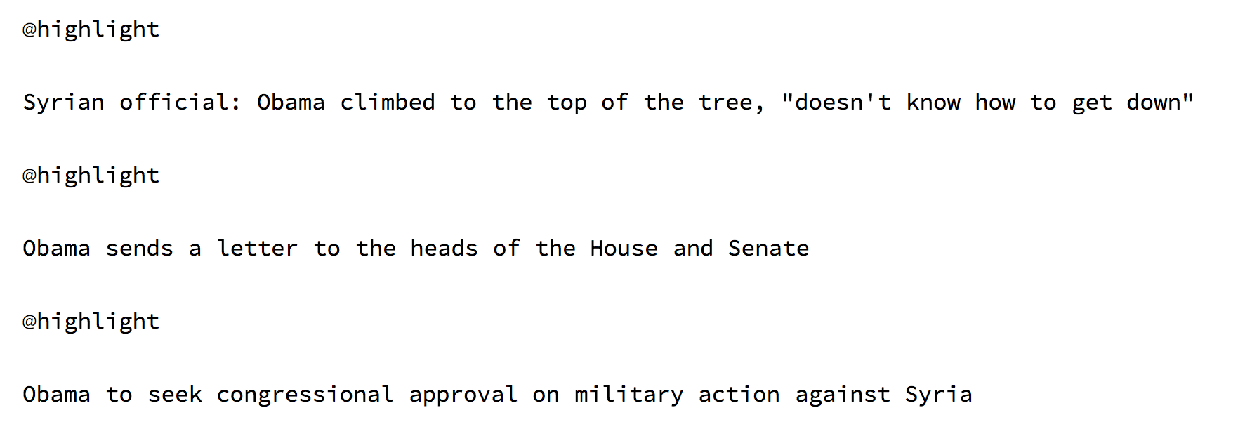
Below there is an example of a story, with the body truncated for brevity.

A number of highlights is appended at the end of each article.

Data Preparation
Data cleaning is always a challenging problem. Since we want to develop a text summarizer, we need to clean the text, which means splitting it into words/sentences and handling punctuation, in order to simplify the learning problem by reducing the size of the vocabulary, and extract better features.
We follow two different approaches to prepare our dataset.
- 1st Approach: Words with Average Length
In the first approach, we consider 1000 words with average length of 6. We split the article into body and highlights, paying attention not to fragment improperly the sentence.
$maxnumchar = 6000; (* 1000 words with average length of 6 *)
processSample[text_] := Module[{parts, story, puncts, maxpos},
    parts = StringSplit[text,"@highlight"];
    story = StringReplace[First@parts, "\n\n"->"\n"];
    If[StringLength[story]>$maxnumchar,
       puncts = Last /@ StringPosition[story, "."|"!"|"?"];
       story=StringTake[story,First @Nearest[puncts, $maxnumchar]];
    ];
    story -> parts[[2]]
];

table=Table[processSample[data[[i]]],{i,1,Length[data]}];
The data, after cleaning, looks like the following one

Then, we split the body and its highlights (target), extracting the highlights.
    startHigh=StringPosition[#, "@highlight"]&/@data;
    extractHigh[text_]:=StringDrop[#,StringPosition[#, "@highlight"][[1,1]]-1]&/@text

    extractedHigh=extractHigh[data];

    target=StringTrim@StringSplit[#,"@highlight\n"]&/@extractedHigh;
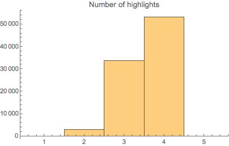
We can count the number of highlights, plotting their frequency in a histogram.
numhighlights=Length[startHigh[[#]]]&/@Range@Length@startHigh;
Histogram[numhighlights, PlotLabel->"Number of highlights"]

- 2nd Approach : "Divide et impera" by paragraphs
The second approach consists in splitting the body into paragraphs and create an association between the paragraph and the highlights. In order to construct an embedding to capture the similarity of the words between paragraphs and summary within the document, we get the pre-trained net Global Vectors (GloVe) , which is based on the Word2Vec method. It allows us to visualize (we can think of an n dimensional space) where each word occupies one of the dimensions. It encodes 1193515 tokens as unique vectors, with all tokens outside the vocabulary encoded as the zero-vector.
word2vec=NetModel["GloVe 100-Dimensional Word Vectors Trained on Tweets"] (* it can be viewed on the Wolfram Neural Net Repository *)
In particular, this neural net processes texts: its input is a text corpus and its output is a set of vectors. The vectors we use to represent words are called word embeddings. In short, word embedding represents a word with numbers, which are natural language computer-readable. The Embedding Layer is useful to encode the sentences by indices, by assigning an index to each unique word.
Now, we create a function to find all unique non - overlapping words from highlights and grab the paragraphs that contain those. First of all, we need to delete the stopwords from the text, because they do not add much meaning to the sentences. We split the text into paragraphs, taking into account its definition (i.e., "a short part of a text that begins on a new line and consists of one or more sentences dealing with a single idea", Cambridge Dictionary). For this purpose, we use the StringSplit[] function, which splits strings into a list of substring separated by delimiters matching the string expression pattern, and the DeleteCases[] function, which removes all elements that match a pattern. Also, we split each paragraph into tokens, specifically into individual words. Therefore, we split each paragraph into tokens, specifically into individual words (note: Stop words are supposed to be in GloVe and GPT-2; however, for a better understanding, we wanted to build a function including an 'external' tokenization). Once we embedded words of both highlights and paragraphs using the net Glove, we can determine the similarity by comparing word vectors in paragraphs and in highlights, and associate one highlight to specific paragraphs by finding its nearest neighbour(s).
processSample2[text_]:= Module[{uniqueHighlightWords,paragraphs,paragraphWords,uniquePositionOfHighlights,uniquePositionOfParagraphs,lookuptable,bestGuess,matches,main,highlights},
{{main},highlights}=StringTrim/@TakeDrop[StringSplit[data,"@highlight"],1];
paragraphs=DeleteCases[StringSplit[main,"\n"],""];
paragraphWords=DeleteStopwords/@StringTrim/@StringSplit/@paragraphs;
uniqueHighlightWords=Table[DeleteStopwords@DeleteCases[StringSplit@highlights[[n]],Alternatives@@StringSplit[StringRiffle[Drop[highlights,n]," "]]],{n,Length@highlights}];
uniquePositionOfHighlights=Mean@Part[word2vec@#,All,1]&/@uniqueHighlightWords;
uniquePositionOfParagraphs=Mean@Part[word2vec@#,All,1]&/@paragraphWords;
lookuptable=AssociationThread[ uniquePositionOfHighlights-> highlights];
bestGuess=Lookup[lookuptable,First/@Nearest[uniquePositionOfHighlights,uniquePositionOfParagraphs]];
matches=Thread[paragraphs-> bestGuess]
]
After that, we save all the data in a binary file, setting the directory to a place for temporary files and saving all definitions by using DumpSave[].
table=Table[processSample[data[[i]]],{i,1,Length[data]}]
SetDirectory[NotebookDirectory[]];
DumpSave["table.mx",table];
Build the Neural Network (GPT-2)
Natural Language processing (NLP) comprises a wide range of tasks such as question answering, semantic similarity assessment, document classification, and text summarization. Recently, OpenAI, a research institute which aims to create artificial intelligence, proposed a model, called GPT-2, a successor to GPT (which stands for Generative Pretrained Transformer). This model was trained to predictive (or generate) the next token in a sequence of tokens in an unsupervised way, by using a transformer architecture. What we need in order to train our model is to load the GPT-2 net.
base = Import["/Users/sadinov/Desktop/GPTcode/net.wlnet"]
The GPT-2 model is trained on large corpora of text (around 1.5 billions of words) on supervised learning tasks. This model outputs a list of numeric vectors, one for each word or subword; these vectors are a numeric representation of the meaning of each word/subword.
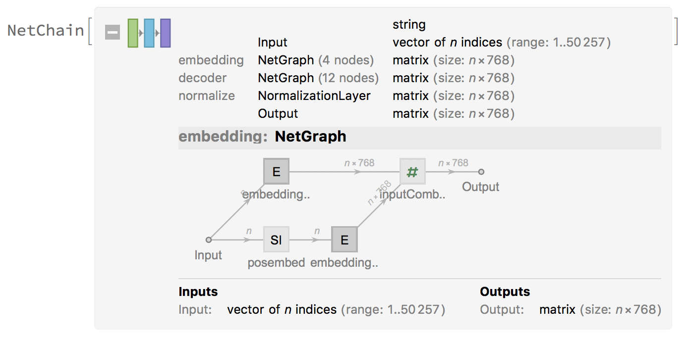
The figures below show the NetChain: it specifies the GPT-2 net in which the output of the i-th layer is connected to the input of the i-th+1 layer. The net takes inputs as a string or vector of n indices and output a matrix nx768. The vocabulary is expanded to 50257.


Most of the common neural networks have three components: an encoder network, a decoder network, and an attention network. The Encoder converts an input document to a feature vector, and the decoder generates a summary by using it. The multi-head attention mechanism allows to model dependencies regardless of their distance in input and output sentence.
The code for the Encoder is the following:
TransformerEncoder[lm_, training_:True, useTokensForPairs_:True] := Module[{ numTokens},
    numTokens = Last@Last@NetExtract[NetReplacePart[lm, "Input" -> Automatic],"Input"];
    With[{
       biSentenceEncoder =
         With[{nt = numTokens},
          With[{
              encoder = NetExtract[lm, "Input"],
              batchify = Function[{func, inputs}, Module[{subref, n, offset, outputs},
                    offset = 0;
                    outputs = func[Flatten[inputs, 1]];
                    Table[
                        n = Length[subref];
                        offset += n;
                        outputs[[offset - n + 1;; offset]]
                    , {subref, inputs}
                   ]
                 ]],
              catenate = Which[
                 training && useTokensForPairs,
                   Function[{tokens1, tokens2}, Transpose[{
                    Join[tokens1, {nt+1}, tokens2, {nt+2}],
                    Join[ConstantArray[1, Length[tokens1]], {1}, ConstantArray[2, Length[tokens2]], {2}]}]
                   ],
                 training,
                   Function[{tokens1, tokens2}, Transpose[{
                    Join[tokens1, tokens2],
                    Join[ConstantArray[1, Length[tokens1]], ConstantArray[2, Length[tokens2]]]}]
                   ],
                 useTokensForPairs,
                   Function[{tokens1, tokens2}, Join[tokens1, {nt+1}, tokens2 (*, {numTokens+2} *)]],
                 True,
                   Join
              ]
          },
              Function[sentences,
                 Map[Apply[catenate], batchify[encoder, sentences]]
              ]
          ]
         ]
       },
       NetEncoder[{"Function",
            biSentenceEncoder,
         {"Varying", If[training, 2, Nothing], Restricted["Integer", numTokens+If[useTokensForPairs,2,0]]},
         "Batched" -> True,
         "Pattern" -> {_String,_String}}
       ]
    ]
]
The code for the Decoder is:
TransformerDecoder[lm_, training_:True, useTokensForPairs_:True] := Module[{tokens, func, encoder},
    func = NetExtract[lm, {"Input", "Function"}];
    encoder = Extract[func,First@Position[func, _NetEncoder]];
    tokens=NetExtract[encoder,"Tokens"];
    If[useTokensForPairs,
       tokens = Join[tokens, {StartOfString, EndOfString}];
    ];
    NetDecoder[{"Class", tokens, "InputDepth" -> If[training, 2, 1]}]
]
As previously said, the NetEncoder[] represents an encoder that takes an input sequence and maps it into a higher dimensional space (n-dimensional vector) representation and decodes it into an expression of a given form. In our case, the input is a matrix of size n x 50259. If used on a probability vector, it can predict the class for a batch of inputs.
enc1=TransformerEncoder[base, True, True]
The generated vector is fed into the decoder. The NetDecoder[] represents a decoder that takes a net representation and decodes it into an expression of a given form.
dec1=TransformerDecoder[base, True, True]
Using the encoder:
encoder = Table[enc1@{table[[i,1]],table[[i,2]]},{i,10}]

The GPT - 2 net has 12 layers, each with 12 independent attention mechanism, called "heads". Having a fast GPU is important to train the model as this allows a rapid gain in results.
LanguageModelNet[basemodel_, useTokensForPairs_:True] := Module[
    {
       embeddingweights, chosenWeightsForNewTokens,
       newembeddingtokens,
       sharedWeights,
       func, encoder, tokens, numTokens, maxNumTokenPosition (* We should not need that with full Automatic inference *)
    },

    func = NetExtract[basemodel, {"Input", "Function"}];
    encoder = Extract[func,First@Position[func, _NetEncoder]];
    tokens=NetExtract[encoder,"Tokens"];;
    numTokens = Length[tokens];

    embeddingweights = NetExtract[basemodel, {"embedding", "embeddingtokens", "Weights"}];
    If[useTokensForPairs,
       (* Add the unknown token weights standing for StartOfString and EndOfString *)
       chosenWeightsForNewTokens = First @ First[
         Position[tokens, "\n"],
         First[Position[tokens, s_String /; StringMatchQ[s, "\n"~~___]],
          First[Position[tokens, "."], {-1}]
         ]
       ];
       Echo["Mapping new tokens to: "<>ToString[tokens[[chosenWeightsForNewTokens]], InputForm]];
       embeddingweights = Echo@NetGraph[
         {
          PartLayer[{chosenWeightsForNewTokens, All}],
          AppendLayer[],
          AppendLayer[]
         },
         {
          {NetPort["Input"], 1} -> 2, {2, 1} -> 3
         },
         "Input" -> Dimensions[embeddingweights]
       ][Echo@embeddingweights];
    ];

    newembeddingtokens = EmbeddingLayer["Weights" -> embeddingweights,
       "Input" -> {"Varying", Restricted["Integer", numTokens+If[useTokensForPairs,2,0]]
    }];
    newembeddingtokens = NetInsertSharedArrays @ newembeddingtokens;
    sharedWeights = First @ Keys @ NetExtract[newembeddingtokens, NetSharedArray[All]];

    maxNumTokenPosition = Last @ Last @ NetExtract[basemodel, {"embedding", "embeddingpos", "Input"}];
    NetChain[
       Join[
         MapAt[
          Function @ NetGraph[
              Join[
                 <|
                   "embeddingtokens"-> newembeddingtokens,
                   "posembed"-> NeuralNetworks`SequenceIndicesLayer[maxNumTokenPosition]
                 |>,
                 Normal[#][[3;;All]]
              ],
              EdgeList[#]
          ]
          , Normal @ basemodel
          , {"embedding"}
         ],
         <|
          "classifier" -> NetMapOperator @ LinearLayer["Weights" -> sharedWeights, "Biases" -> None]
          , "softmax" -> SoftmaxLayer[]
         |>
       ]
       , "Input" -> TransformerEncoder[basemodel, False, useTokensForPairs]
       , "Output" -> TransformerDecoder[basemodel, True,  useTokensForPairs]
    ]
]
In order to improve the performance, we consider the Teacher Forcing as approach. The Teacher Forcing is a method for efficiently training neural network models that use model output from a prior time step as the next input. Teacher forcing works by using the actual or expected output from the training dataset at the current time step y(t) as input in the next time step x(t + 1), rather than the output generated by the network, and this allows the models to converge faster.
If we look at the following code, we can see that the SequenceRestLayer[] represents a net that takes a sequence of inputs and removes its first element. SequenceMostLayer[] represents, instead, a net that takes a sequence of inputs and removes its last element. These layers are implemented for generation of previous and next token, but also to generate the next sentence. This means that, given our dataset containing a sequence of sentences, the decoder is expected to generate the previous and next sentences, token by token. The encoder - decoder network is trained to minimize the sentence reconstruction loss and the encoder learns to generate vector representations.
TeacherForcingNetWithWeighting[lm_, useTokensForPairs_:True] := NetGraph[
    <|
       "LM" -> LanguageModelNet[lm, useTokensForPairs],
       "token" -> PartLayer[{All, 1}], (* word encoder *)
       "previous-token" -> SequenceMostLayer[],
       "next-token" -> SequenceRestLayer[],
       "sentence" -> PartLayer[{All,2}], (* sentence encoder *)
       "next-sentence" -> SequenceRestLayer[],
       "weight" -> ElementwiseLayer[1.00001*(#-1)&(*, "Input" \[Rule] {"Varying",Restricted["Integer", 50257]}*)],
       "losses" -> NetMapThreadOperator[CrossEntropyLossLayer["Index"]],
       "weightedlosses" -> ThreadingLayer[#1 * #2&],
       "totalloss" -> SummationLayer[] (* AggregationLayer[Total, 1] *)
    |>,
    {
       NetPort["Input"] -> "token" -> {"next-token", "previous-token"},
       NetPort["Input"] -> "sentence" -> "next-sentence" -> "weight",
       "previous-token" -> "LM",
       "LM" -> NetPort["losses", "Input"],
       "next-token" -> NetPort["losses", "Target"],
       {"weight", "losses"} -> "weightedlosses" -> "totalloss" -> NetPort["Loss"]
    },
    "Input" -> TransformerEncoder[lm, True, useTokensForPairs]
];
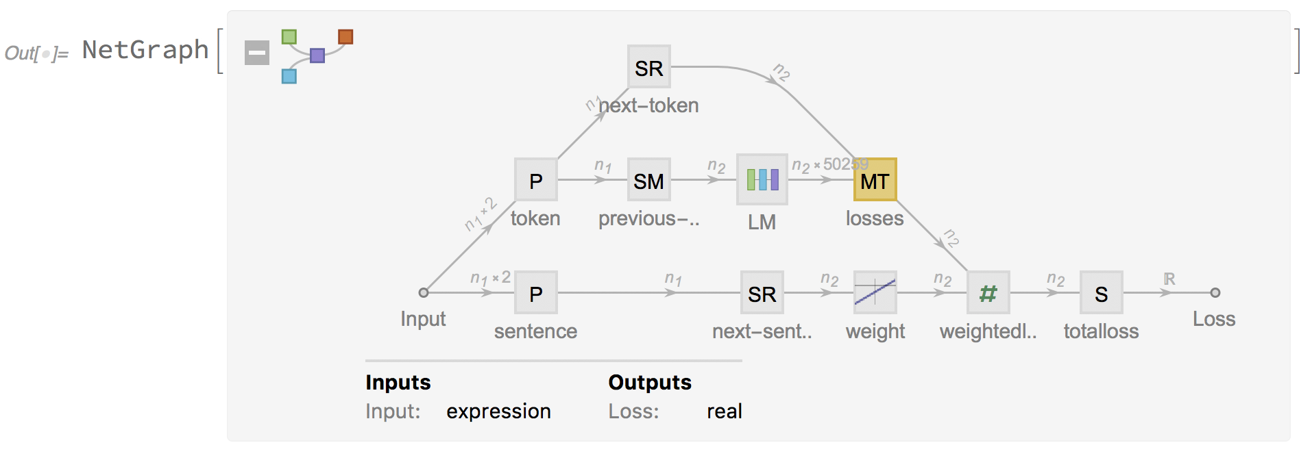
Let us take a look at the NetGraph[]. Neural networks are trained using an optimization process that requires a loss function to calculate the model error. The cross - entropy and mean squared error are the two main types of loss functions to use when training neural network models. In particular, the CrossEntropyLossLayer[] represents a net layer that computes the cross - entropy loss by comparing input class probability vectors with indices representing the target class.
lmteacherforcing = TeacherForcingNetWithWeighting[base,True]

Net Train
The following is the code for running the Neural Network Training on GPUs/Multiple GPUs.
trainednet = NetTrain[
    lmteacherforcing
    , <|"Input" ->  Table[{table1[[i,1]],table1[[i,2]]},{i,10000}]|>
    (*, All*)
    (*, ValidationSet -> Scaled[0.2] *)
    , LossFunction -> "Loss" (*lossSpec*)

    , TrainingStoppingCriterion -> <|
       "Criterion" -> "Loss"
       , "Patience" -> 10
    |>
    , MaxTrainingRounds -> Quantity[1 * 10 * 60 * 60, "Seconds"]

    , BatchSize -> 16 (* 512 *)
    , LearningRateMultipliers -> {{"LM", "embedding"} -> None} (* 0.07*)

    , TrainingProgressCheckpointing -> {
       (*"Directory", dirname,*)
       "File", outputFilenameTrainer,
       "Interval" -> Quantity[600,"Seconds"]
       (*, "Format" -> If[hasFrozenLayers, "params", "wlnet"]*)
    }
    , TrainingProgressReporting -> {
       File @ outputTrainingLog, "Interval" -> checkInterval
    }

    , TargetDevice -> {"GPU", All}
];
We can set a checkpoints folder to save the entire folder and start off with the previous saved checkpoint.
Future Work
Future work would investigate methods to optimise the neural network architecture, in order to achieve more accuracy on different datasets and topics. Another possible direction would be to improve the robustness of Deep Learning Model by adding noise.
References
- A. Radford, J. Wu et al., Language Models are Unsupervised Multitask Learners, 2019
- S. Narayan, N. Papasarantopoulos et al., Neural Extractive Summarization with Side Information, 2017
- S. Narayan, N. Papasarantopoulos et al., Neural Extractive Summarization with Side Information, 2017
- J. Li, M-T- Luong et al., A Hierarchical Neural Autoencoder for Paragraphs and Documents, 2015
- M. Kageback,O. Mogren, Extractive Summarization using Continuous Vector Space Models, 2014
- L. Shifrin, Mathematica Programming: An Advanced Introduction, 2008
Links
- https://github.com/openai/gpt
- https://resources.wolframcloud.com/NeuralNetRepository/
- http://www.wolfram.com/language/fast-introduction-for-programmers/en/
Contact: