Aggregation System of a Totalistic Rule
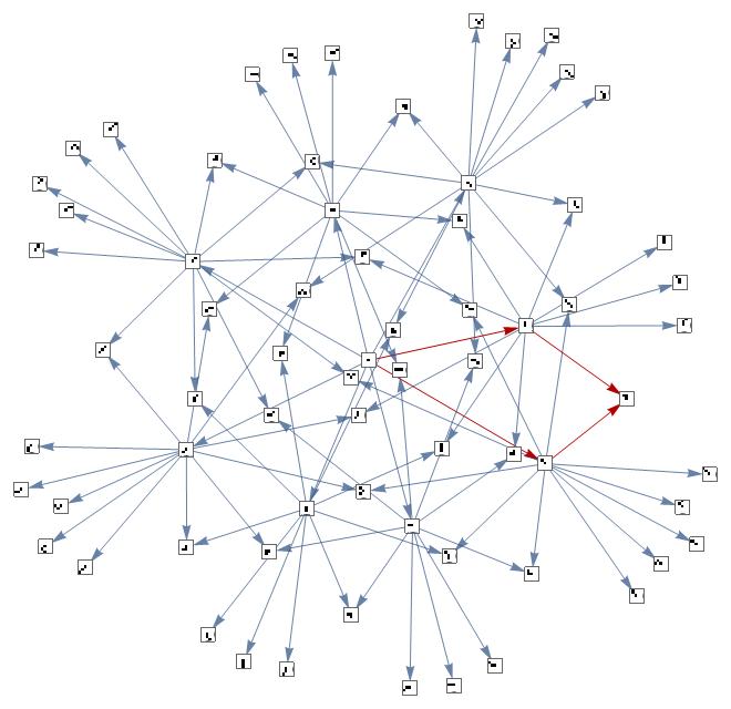
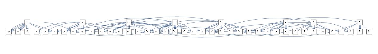
All possible paths the Aggregation System can take
Introduction
Aggregation Systems are a stochastic analog to the Cellular Automaton. Unlike Cellular Automaton, where every step is deterministic and it grows one row at a time, Aggregation Systems grow by adding one cell at a time at randomly chosen locations. But at the same time, there are certain underlying rules similar to the Cellular Automaton rules they follow. So, it is random but has a deterministic tinge of the Cellular Automata rules. For example, one step of Rule 30 in CA and AS,
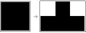
Rule 30 CA
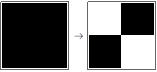
Rule 30 AS
As you can see, the Aggregation System model basically follows the rules of the Cellular Automaton but instead of adding all the cells in the following row, it picks one at random. After around 30 steps, this is how they both look (Rule 30 of elementary Cellular Automaton).
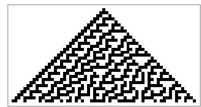
CA
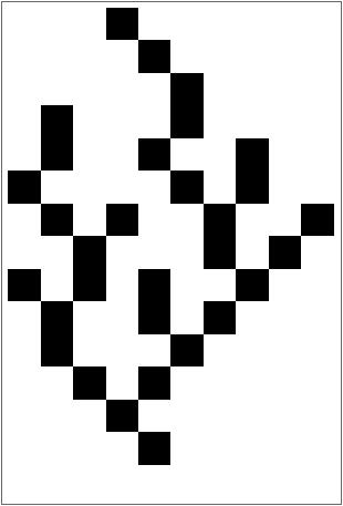
AS
A lot of "random" behavior of nature could be modeled using the Outer Totalistic and Totalistic Rule Set of the Aggregation System and hence, most of the results in the following post are calculated for the Outer Totalistic Case (2D) with an initial condition of an array with one black cell at the center.
Aggregation System Function
Clear[framedAggregationSystem];
framedAggregationSystem[rule_, init_, steps_]:= Catch[Module[{r, p, pos, output1},Nest[
(
r=CellularAutomaton[rule,#];
pos= Position[r, Except[0], {Depth[init]-1}, Heads->False];
If[pos=== {}, Throw[#]];
p=RandomChoice@pos;
output1 = ReplacePart[#,p-> Extract[r, p]]
)&,init,steps]]]
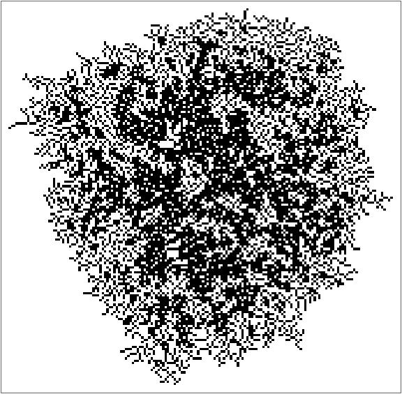
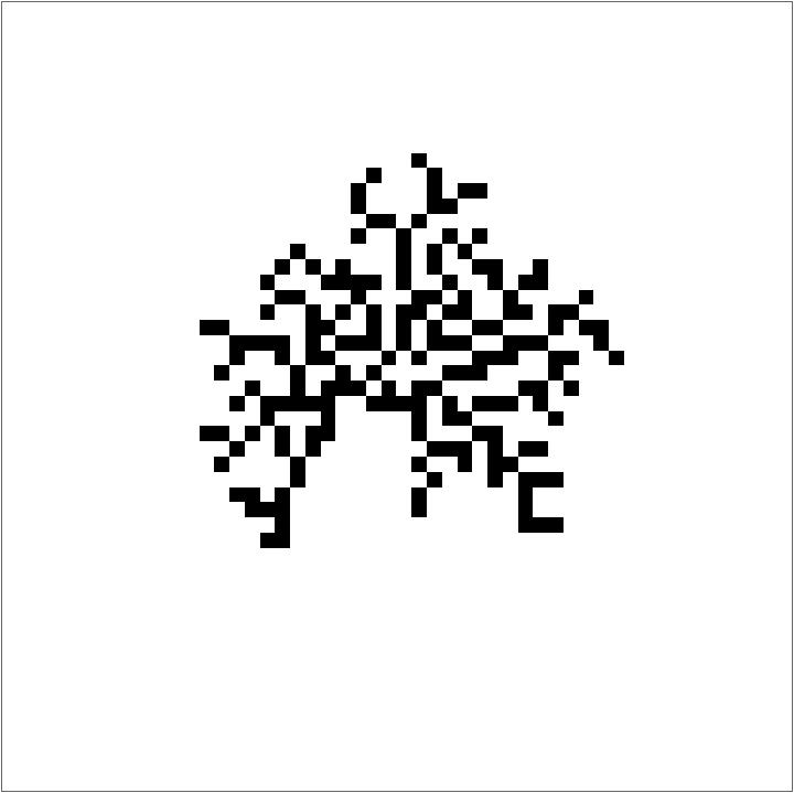
Running this code for Outer Totalistic Rule # 30, gives an image something like this:
Efficient implementation of the same
But this algorithm is inefficient because one needs to define an arbitrary size of the frame to fit the Aggregation System and the algorithm goes on evaluating the white background cells even when the Aggregation System dies down. The next step was to overcome this issue. For that, I evaluated each step of the Aggregation System and evolved the frame accordingly along with the frame. So I pad the initial condition, evaluate the rule and blacken the cell, and then unpad if needed. Here's the code for that:
unpad[a_]:=(ReplacePart[a,Thread[(Replace[#,All->_,1]&/@Select[Catenate@Table[Append[ConstantArray[All,n],m],{n,0,Depth[a]-2},{m,{1,-1}}],AllTrue[Flatten[Extract[a,#]],#===0&]&])->Nothing]])
Clear[AggregationSystem];
AggregationSystem[rule_, init_, steps_]:= Catch[Module[{r, p, pos, output1,output2,cent=0},Nest[
(output1=ArrayPad[#,1];
cent+=1;
r=CellularAutomaton[rule,output1];
pos= Position[r, Except[0], {Depth[init]-1}, Heads->False];
If[pos=== {}, Throw[#]];
p=RandomChoice@pos;
output1 =output2= ReplacePart[output1,p-> Extract[r, p]];
output1=unpad[output1];
output1
)&,init,steps]]]


ArrayPlot@AggregationSystem[<| "OuterTotalisticCode"-> 30 , "Dimension"-> 2|>, CenterArray[1, {1,1}], 200]
Running rule 30 with this:
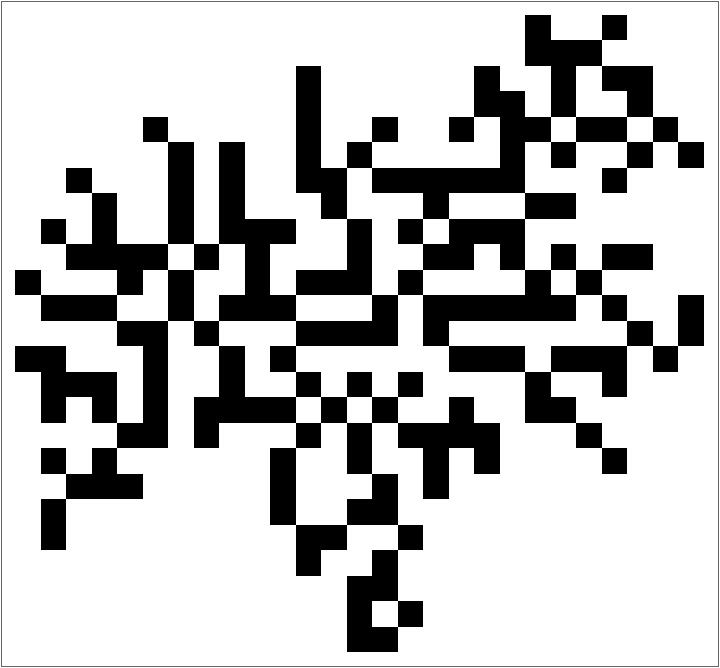
This makes it highly efficient:
TIme vs iterations of both the algorithms
Overview of the rules
The space of outer totalistic rules is about 262143. But odd rules are uninteresting as they flicker and some rules simply do not grow given the initial condition of the Center Array. Eliminating them, I was left with 65536 rules which are still large. One of the brute force ways to get some intuition and understanding about which directions to look for is to simply run all the rules and stare at them:

First 100 Outer Totalistic Rules for about 200 iterations
TESTS AND EXPERIMENTS
Dimensions
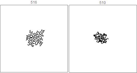
If one stares at the rules for a while, you realize that there is some sort of burst in the dimensions after a certain discrete rule number. This hints towards behavior during systems where there is a phase change of some sort. For example, rule 510 ->516:
This happens all the time and is not by chance. Iterating each rule 20 times and plotting the dimensions:
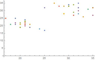
X and Y coordinates of rules 510 and 516 when run multiple times.
In other words, this is the result of the tinge of determinism in the rules of the Cellular Automaton applied to "random" Aggregation Systems.
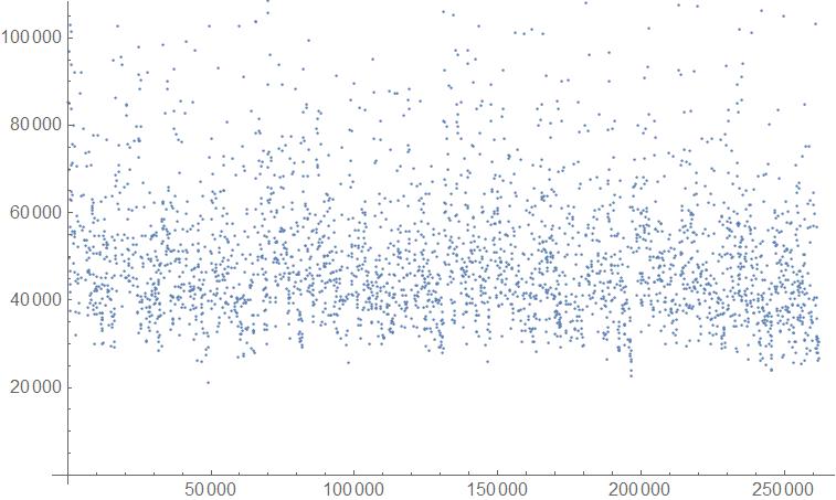
Plotting the dimensions for the whole rule space of Outer Totalistic:
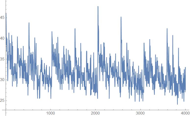
The spikes mainly occur around the powers of 2 because that is where the rules undergo a major change in terms of the number of cells turning to black given a neighborhood.
Standard Deviation
On iterating each rule a several number of times, I got a different picture almost every time as the cells are picked one at a time from a set of finite possible options. This raises the question of whether there exists some sort of a behavioral characteristic to a rule we can predict beforehand given the rule number. One of the measures to look at it is the Standard Deviation of the pixel values {0,1} after iterating a rule for a fixed number of iterations. So given, the number of iterations for each rule and the number of rules we want this result for, here's the function that gives the standard deviation of the cell values:
available =  Select[Range[2^18-1],EvenQ[#] &&!IntegerQ[#/8]&&!IntegerQ[(#-10)/8]&];
stdeviationrandomavailable[iterations_, n_]:=
( a = RandomSample[available, n];
KeyValueMap[N@StandardDeviation@#2&,Merge[Table[AssociationMap[AggregationSystem[<| "OuterTotalisticCode"-> # , "Dimension"-> 2|>, CenterArray[1, {50,50}], 500]&, a], {k,iterations}],Identity]]
)
AssociationThread[a, ArrayPlot/@stdeviationrandomavailable[10, 5]]
Output:
Doing the same for a higher iteration value:
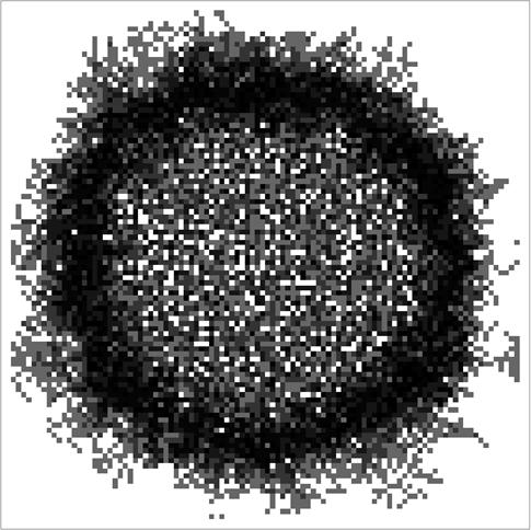
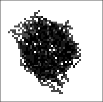
I noticed that many of the rules have a dark halo at the edges. This happens because when we run a rule a multiple number of times, the inner section almost remains the same; like a dense blob. Only at the outer parts of the system that there is an uncertainty of the positions of the cells leading to a higher standard deviation. But this is not always true as one would normally expect. For example, Rule 2143:
In this case, there is uncertainty engraved in the rule from the very beginning and the standard deviation plot almost looks like a black blob. If we go on to plot something analogous to the moment of inertia in that case of these Standard deviation visuals (vs Rule Number), we get an idea as to what is the distribution of the two types of Standard Deviation representations.
datastdev = Import["stdeviationdata.mx"];
ListPlot@AssociationThread[labels, Table[N[Total[Flatten@MapIndexed[#1*(EuclideanDistance[Dimensions[datastdev[[n]]]/2,#2]^2)&,datastdev[[n]],{2}]]], {n, 1, 3000}]]
Histogram:
Histogram[AssociationThread[labels, Table[N[Total[Flatten@MapIndexed[#1*(EuclideanDistance[Dimensions[datastdev[[n]]]/2,#2]^2)&,datastdev[[n]],{2}]]], {n, 1, 3000}]]]
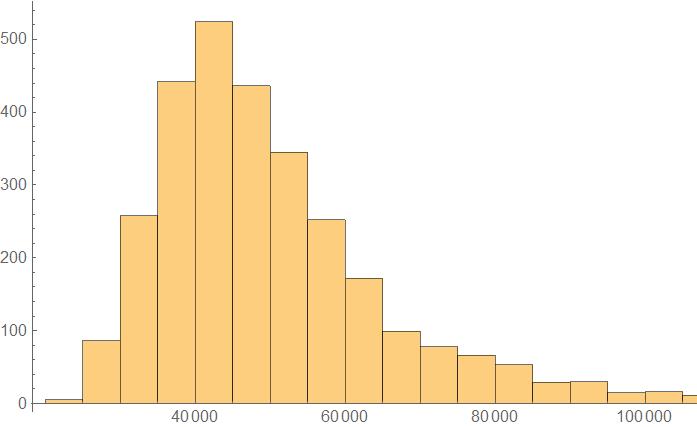
On looking for the distribution,
FindDistribution[Table[N[Total[Flatten@MapIndexed[#1*(EuclideanDistance[Dimensions[datastdev[[n]]]/2,#2]^2)&,datastdev[[n]],{2}]]], {n, 1, 3000}]]
we get the following:
MixtureDistribution[{0.9262480618395671, 0.07375193816043307}, {LogNormalDistribution[10.709938521692017, 0.24927531644683798], LogNormalDistribution[11.375808011619768, 0.3116990014250025]}]
Mean
Another thing that comes to mind after Standard deviation is the mean of the rules after iterating multiple times. Similar to the standard deviation, here's the code for the mean calculations:
meanrandomavailable[n_, iterations_]:=
(a = RandomSample[available, n];
KeyValueMap[ArrayPlot[N@Mean@#2, PlotLabel-> #1]&,Merge[Table[AssociationMap[AggregationSystem[<| "OuterTotalisticCode"-> # , "Dimension"-> 2|>, CenterArray[1, {45,45}], 200]&,a], {k,iterations}],Identity]])
meanrandomavailable[10,10]
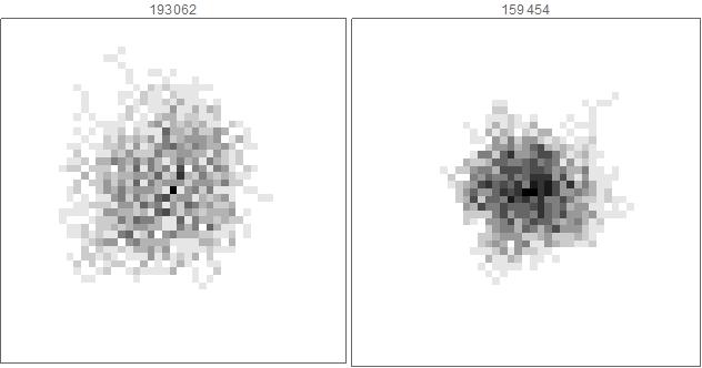
This again tells us about the characteristic of rules. Certain rules like 159454 have a Gaussian distribution implying that they're more likely to land in that particular spot than in other places. On the other hand, some rules like 193062 are by and large of the same probability everywhere implying that a cell is equally likely to land in any given area. They display a dispersed behavior in comparison to the rules like 159454.
Confluence
Confluence is essentially a property of a rewrite system which indicates whether or not a system (observed) can be transformed or rewritten in a way that the input of an abstract rewrite pair overlaps to the same result after the following iteration. If this happens over a single rewrite rule iteration for all given states of a system, the system is said to be locally or weakly confluent and the system is said to display the Church-Rosser property. If this, occurs over multiple transformation steps, the system is said to be globally confluent. Confluence is usually studied in deterministic systems and the study of confluence hasn't really been taken up in stochastic systems. Here, I aim to bring up an idea of confluence in the case of these stochastic Aggregation Systems.
"Theoretical" evaluation of Confluence Levels
Given an initial condition of the Center Array and a rule, there are different states in which a system can evolve to. Some of these states can be further evolved to converge into the same state. For example,
Code for the above:
Clear[DeterministicAggregationSystem];
DeterministicAggregationSystem[rule_, init_]:= Catch[Module[{r, pos},Nest[
(
r=CellularAutomaton[rule,#];
pos= Position[r, Except[0], {Depth[init]-1}, Heads->False];
If[pos=== {}, Throw[#]];

Function[p,ReplacePart[#,p-> Extract[r, p]]]/@pos
)&,init,1]]
]
The above fuction lists all the possible states from one iteration to the other.
removeSelfLoops[g_Graph]:=Graph[DeleteCases[EdgeList[g],(DirectedEdge|UndirectedEdge)[x_,y_]/;x===y],Sequence@@Options[g]]
theoreticalconfluencegraph2[rule_,iters_,initI_:CenterArray[1,{5,5}]]:=Module[{graphint},
graphint = Graph[Labeled[#,#,Center]&/@VertexList[#],DeleteDuplicates@EdgeList[#]]&@Graph[
Catenate[Module[{newInit},Reap[Nest[
Catenate@*Map[Function[init,
newInit=DeterministicAggregationSystem[rule,init];
Sow[ArrayPlot[init,ImageSize->15]\[DirectedEdge]ArrayPlot[#,ImageSize->15]&/@newInit];
newInit
]],
{initI},iters];
]][[2,1]]]
];
removeSelfLoops[graphint]
]
g = theoreticalconfluencegraph2[<| "OuterTotalisticCode"->30, "Dimension"-> 2 |>, 2];
g = HighlightGraph[g, {ReplacePart[VertexList[g][[{1,2}]],0->DirectedEdge]}];
g = HighlightGraph[g, {ReplacePart[VertexList[g][[{2,14}]],0->DirectedEdge]}];
g = HighlightGraph[g, {ReplacePart[VertexList[g][[{1,3}]],0->DirectedEdge]}];
g = HighlightGraph[g, {ReplacePart[VertexList[g][[{3, 14}]],0->DirectedEdge]}]
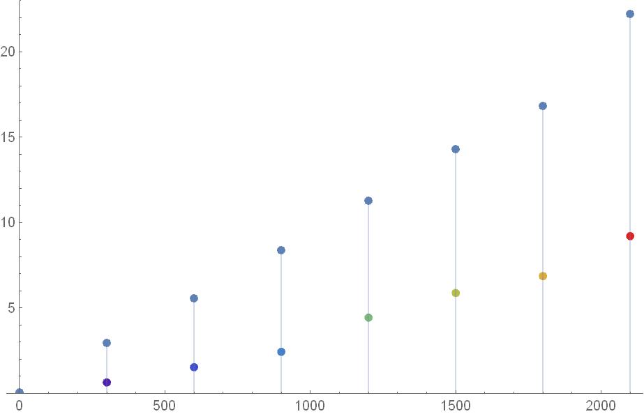
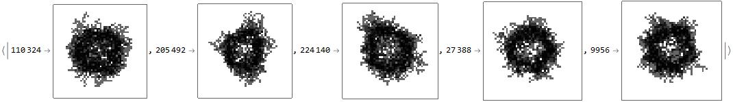
The highlighted part of the graph is one of the possible paths that can be taken by the system that converge after two iterations. We calculate the probability of achieving such states since these bring the confluence to the rule. For example, there is a {1/80, 1/80 } chance to take those paths on multiple iterations. Then, we go on to calculate such probabilities for all such convergent states and take the sum. This, in essence, defines a theoretical confluence level of a particular rule.
theoreticalconfluencevalue [graph_]:=
(Module[{val, probs},probs = Select[AssociationMap[Apply[Function[{v1,v2},Function[path,1/Times@@(VertexOutDegree[graph,#]&/@Most[path])]/@FindEdgeIndependentPaths[graph,v1,v2,Infinity]]],Permutations[VertexList[graph],{2}]],Length[#]>1&];
Print[probs];
val = N[Total@Flatten@Values@probs]
])
theoreticalconfluencevalue[g]

Output confluence value: 0.641667
Experimental Evaluation of weak confluence
Until now, we algorithmically defined and calculated the theoretical confluence level of a given ruleset. But the speculation is that this might not be so simple after all and it is a good idea to compare it to the real Aggregation System by actually running it and fetching raw data.
Algorithm and evaluation
Given a rule set and the initial condition of the central array, two iterations of the Aggregation Systems are evaluated for a certain sample number of times (200+) and displayed as a graph. To get the confluence level in the ruleset, we first count the number of pairs of edges that point to a particular state in the second iteration from non-overlapping first iterations. We then divide this number by the total number of "VertexOut" edges from the corresponding first iteration states. Finally, if this occurs for multiple states in the second iteration, the ratios are independently added and the resulting value is the experimental confluence level of the ruleset.
confluencegraph[rule_, iter_]:=(Module[{step1, step2, g, confgraph},
step1=Table[AggregationSystem[<| "OuterTotalisticCode"-> rule, "Dimension"-> 2 |>,CenterArray[1, {10, 10}], 1], {i, iter}];
step2 = Table[AggregationSystem[<| "OuterTotalisticCode"-> rule, "Dimension"-> 2 |>,step1[[i]], 1], {i, iter}];
g=Graph[Flatten[{
Thread[DirectedEdge[(ArrayPlot[#,ImageSize->20]&/@step1),(ArrayPlot[#,ImageSize->20]&/@step2)]]
}]];
confgraph = removeSelfLoops@Graph[Labeled[#,#,Center]&/@VertexList[g],EdgeList[g]]
])
confluencevalue[graph_Graph]:=Module[{keys, inOutDegree, exprob},
(keys=Keys@countofpairs[graph];
inOutDegree=AssociationMap[AssociationMap[VertexOutDegree[graph,#]&,DeleteCases[VertexInComponent[graph,#,1],#]]&,keys];
exprob=Merge[{countofpairs[graph],Total/@inOutDegree},#[[1]]/#[[2]]&];
Total[exprob])]
experimentalconfluencegraph = confluencegraph[100, 100]
confluencevalue[experimentalconfluencegraph]//N
Output Confluence Value: 1.24847
Conclusion
A function was successfully fabricated to give out the Aggregation System given the rule number, initial conditions, and the number of iterations (exactly like Cellular Automaton). Following that, the function was made efficient by precisely fitting it to the frame. Then, certain properties like dimensions, standard deviation, and mean were studied which revealed some behavioral patterns which hint towards natural events like phase changes in a system. Finally, the study of confluence, which is usually done on a deterministic system, was undertaken giving statistics on the "confluenciality" of a stochastic model of this type.
Future Work
- Extending the function to include 3D Aggregation Systems.
- Extending similar studies to a general space of initial conditions and other rule sets.
- Looking for interesting patterns by analyzing parameters like fractal box dimension, growth of the system with time, etc.
- Continue investigations on confluence in the rule space and look for stronger results.
 Attachments:


