Mentor: Jonathan Gorard
GitHub
We examined confluent set substitution systems using SetReplace package. We specifically obtained three results. First, we looked into applying critical pair completion idea from automated theorem proving to get quantum behavior. We did not explicitly reproduce any quantum effects, however, we found several possible directions to explore. Second, we emulated elementary cellular automata with non-overlapping set substitution systems, which demonstrates their universality.
Critical Pair Completion
Confluence and Relativity
In rewrite systems, the reference frame is determined by the order of rewrite events [NKS, 516]. In general, different order of rewrite events will yield different states of the system (i.e., rewrite events do not commute), which, at least if one only considers a single branch of the multiway system, does not reproduce special relativity.
To get around this issue, one idea is to only consider confluent rewrite systems, i.e., rewrite systems in which every divergent pair of rewrites (critical pair) can be converged to a single branch.
Furthermore, due to Newman's lemma [Newman, 1942] local confluence is equivalent to global confluence, i.e., the possibility of converging a critical pair immediately is both sufficient and necessary for the global confluence (and therefore relativistic-ness) of the system.
One approach that is explored more in the next section is to begin with a rule that is locally confluent. However, in this section we explore a different approach based on real-time critical pair completion.
Critical Pair Completion for Strings
Critical pair completion is an idea from automated theorem proving, where one starts evolving an arbitrary rewrite system as usual, but as soon as a critical pair is encountered, one adds a new bi-directional rule between the critical pair outputs.
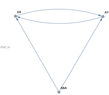
For the sake of demonstration, consider the following non-confluent string rewrite system:
In[] := StringReplaceList["ABA", {"AB" -> "X", "BA" -> "Y"}]
Out[] = {"XA", "AY"}
Note the critical pair arises because there are two ways to make a substitution, and once made, the system terminates. One can however add new rules to deal with this:
{"XA" -> "AY", "AY" -> "XA"}
Now, the multiway network of this system is confluent, as there is a way to get from any final state to any other state
In[] := NestGraph[
 StringReplaceList[#, {... (*original rules*), ... (*new rules*)}] &, "ABA", 2, ...]
Critical Pair Completion for Networks
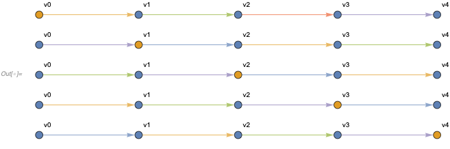
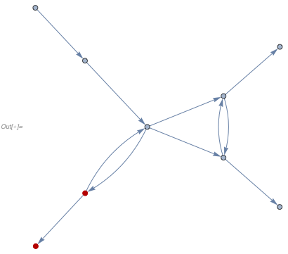
A similar approach can be used with networks. Consider for instance a particle represented as a single-vertex edge moving on a path graph.
In[] := {{v0}, {v0, v1}} -> {{v1}, {v0, v1}} // ... (* HypergraphPlot *)

In[] := SetSubstitutionSystem[... (* rule *),
   {{v0}, {v0, v1}, {v1, v2}, {v2, v3}, {v3, v4}},
   4] // ... (* HypergraphPlot *)
This system is confluent already, in fact its multiway system is
In[] := multiwayGraph[... (* rule *), ... (* path graph *), 4, ...]

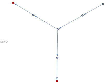
But what if we have a branching in the graph? What if we start with the initial condition
In[] := {{v0}, {v0, v1}, {v1, v2}, {v2, v3}, {v3, v4}, {v2, v5}, {v5, v6}} //
   ... (* HypergraphPlot *)
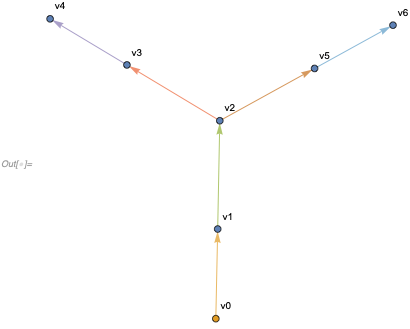
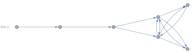
We then get a multiway system with two branches
In[] := multiwayGraph[... (* rule *), ... (* branching graph *), 4, ...]
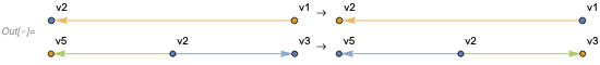
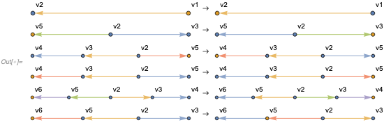
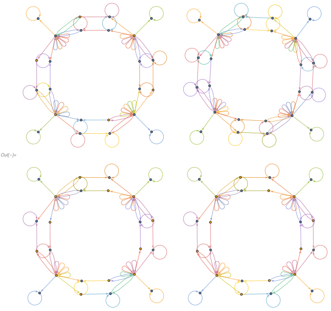
If we now perform a critical pair completion, we get an extra rule to move the particle back and force between branches
In[] := branchCollapseRules[
  multiwayGraph[ ...], { ... (* rule *)}] // ... (* HypergraphPlot *)
and the multiway system becomes
In[] := multiwayGraph[
 branchCollapseRules[ ...], ... (* branching graph *), 4, ...]
Note, a single collapse is insufficient to produce a confluent system, we need to perform a collapse again. After the next iteration we get
In[] := Nest[branchCollapseRules[
    multiwayGraph[#, ... (* branching graph *), 4], #] &,
  ... (* original rule *), 2] // ... (* HypergraphPlot *)
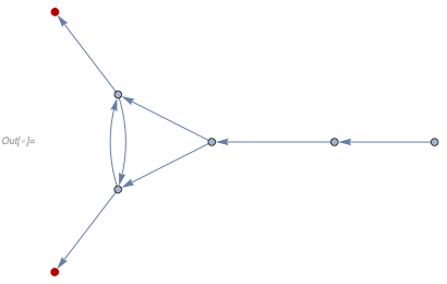
with the multiway system
In[] := multiwayGraph[
 Nest[ ... (* branch collapse rules *)],
  ... (* branching graph *), 5, ...]
Note an interesting point that the rules created at this step allow one to go "back in time". The loop created by this does not constitute a problem as it is not an actual time loop (in a sense of the causal network), but an evaluation loop, which the observer existing in any of the states of the system cannot see.
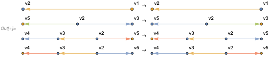
If we keep collapsing critical pairs until the fixed point, we will get the following rules
In[] := FixedPoint[
  branchCollapseRules[
    multiwayGraph[#, ... (* branching graph *), 4], #] &,
  ... (* original rule *)] // ... (* HypergraphPlot *)
and the multiway system that is a complete graph
In[] := multiwayGraph[
 FixedPoint[ ... (* branch collapse rules *)],
  ... (* branching graph *), 5, ...]
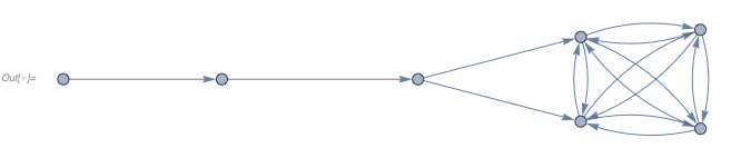
Note the multiway system we get after the first branching point is a complete graph. That is in fact a general feature. At first sight that seems like an issue, because the multiway graph loses all structure, therefore we don't gain anything by performing critical pair completion.
"Quantum" States
However, one has to realize that the rules used for completion are slightly more general than necessary to collapse the branches, and as such they might produce new states that did not exist in the system with original rules.
To see this happen, consider a graph with a branch that is not accessible in the original (classical) system
In[] := {{v0}, {v0, v1}, {v1, v2}, {v2, v3}, {v3, v4}, {v2, v5}, {v5,
   v6}, {v7, v2}, {v7, v8}, {v8, v9}} // ... (* HypergraphPlot *)
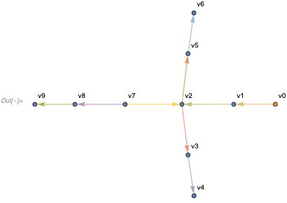
In this system, the particle can never be at v7, v8 or v9 because they are not accessible by following directed edges from v0. However, after a single critical pair completion we get the multiway system that "leaks" into the forbidden branch
In[] := With[{multiway =
   multiwayGraph[
    Nest[ ... (* branch collapse rules *)],
      ... (* graph with inaccessible path *), 5, ...]},
 HighlightGraph[multiway,
  Complement[VertexList[multiway],
   VertexList[multiwayGraph[ ... (* original rules *)]]]]]
This effect exhibits some similarity to quantum tunneling, in a sense that we can get classical-looking states which are nevertheless not accessible from the original system.
However, more investigation of more realistic systems is necessary to, for example, compare probabilities (which are not even clear how to compute in this model) of tunneling to what we expect from quantum mechanics.
Other Ideas
A notable feature of the systems considered above is that multiway systems with original rules might significantly diverge. If one thinks of the original systems is classical, it would be plausible, for example, for the Earth to exist and not exist on different branches. Which essentially implies many-worlds interpretation of Quantum Physics. In other words, observer's memory is different on different branches.
Another possibility is that all branching disappears by the observer's scale, and the observer essentially sees the course-grained version of the multiway system.
In the description of "tunneling" above, we considered the first possibility. In what follows, we will only examine non-overlapping systems, which is the simplest case of the second possibility.
Simulating Cellular Automata
Problem Definition
To begin our study of non-overlapping systems, we will demonstrate their universality by simulating rule 110 elementary cellular automaton (CA) with it.
Rule 110 if started with a single black cell produces a collection of interacting structures
In[] := ArrayPlot[CellularAutomaton[110, {{1}, 0}, 500], ...]
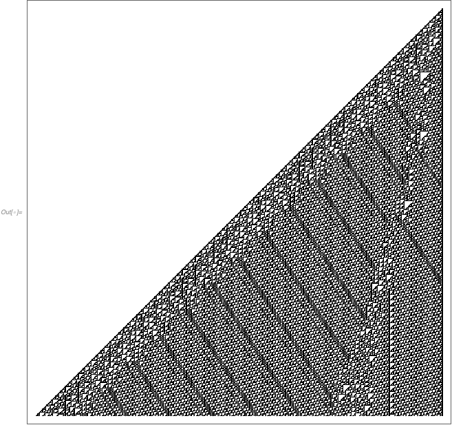
One can in fact use these interacting structures to demonstrate its universality [NKS, 675].
We will use this fact to in turn demonstrate the universality of non-overlapping set substitution systems.
Finite Grid Cells Representation
We begin by simulating a CA with a finite grid. To achieve that we begin with a schematic representation of a CA cell
caBlock[id_String, neighborIDs_ : {_String, _String},
  color_Integer] := {
   {cellCenter[id], "nextStepLeftNeighborInput",
    nextStepLeftNeighborInput[id]},
   {cellCenter[id], "nextStepRightNeighborInput",
    nextStepRightNeighborInput[id]},
   {cellCenter[id], "nextStep", nextStepCenter[id]},
   {cellCenter[id], "inputFromLeftNeighbor",
    rightNeighborInput[neighborIDs[[1]]]},
   {cellCenter[id], "inputFromRightNeighbor",
    leftNeighborInput[neighborIDs[[2]]]},
   {cellCenter[id], color},

   {leftNeighborInput[id], "nextStep",
    nextStepLeftNeighborInput[id]},
   {leftNeighborInput[id], color},

   {rightNeighborInput[id], "nextStep",
    nextStepRightNeighborInput[id]},
   {rightNeighborInput[id], color}
   } // Map[ToString, #, {2}] &
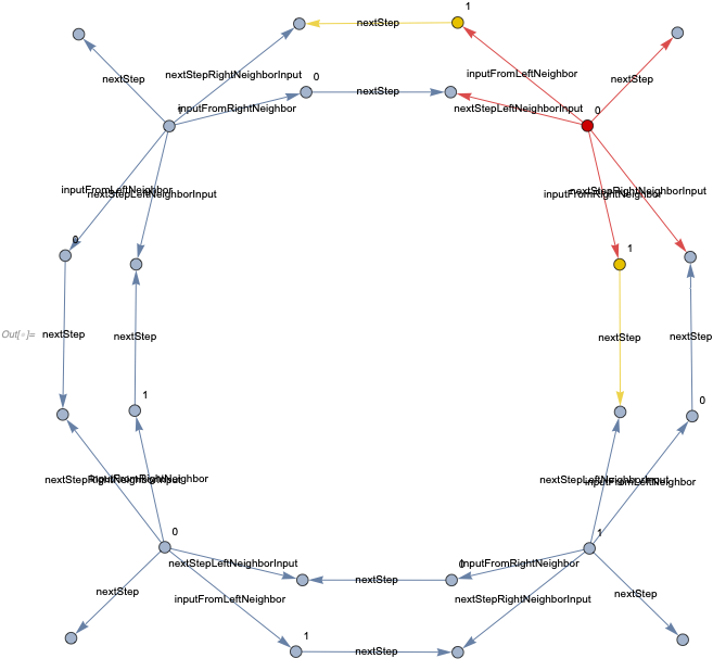
For a finite grid with 4 cells 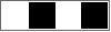 we get the following structure, where a subgraph corresponding to the first cell is highlighted in red, and its connections to the neighboring cells are in yellow.
In[] := Join[caBlock["0", {"3", "1"}, 0], caBlock["1", {"0", "2"}, 1],
  caBlock["2", {"1", "3"}, 0],
  caBlock["3", {"2", "0"}, 1]] // ... (* HypergraphPlot *)
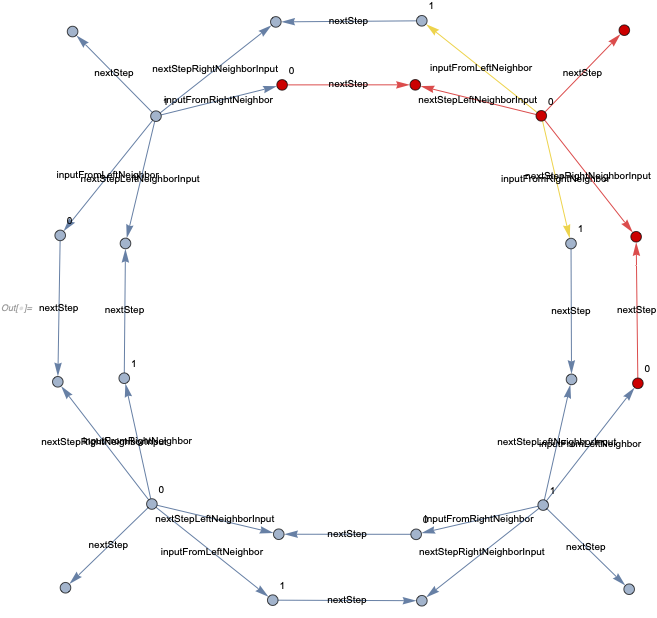
Note there are 6 vertices used to represent each cell: there are three colored ones for the current step. Out of these three, one is used to determine the color at the next step for the current cell, and two others are used by neighbors. Three other cells correspond to the cell at the next time step, and are not assigned any color.
Color Updating Rules
We can then make a rule that would take as an input
Note there is no overlap between different rule applications (some vertices are not highlighted because we are only concerned with the overlap of edges here, and as vertices at the next step do not carry any information, we do not need to associate any additional edges to them apart from highlighted references).
These rule inputs have 5 tentacles going from the main (middle) cell vertex: three point to the next time-step representation of the same cell, and at the rule application, they need to be assigned a particular color.
The other two point to the next step of the neighbors. The vertices these tentacles point to would not be updated, however, the references for the next step would be moved to the next steps of the neighbors (also blocking subsequent updates from happening until neighbors are updated as there is no color initially assigned to the next steps of the neighbor cells).
We can schematically write the rules as
caRules[rule_Integer] :=
  With[{oldLeft = #[[1]], oldMiddle = #[[2]], oldRight = #[[3]],
      newColor = #[[4]]}, {
       {cellCenter_, "inputFromLeftNeighbor",
        leftColorReference_}, {leftColorReference_, "nextStep",
        nextStepLeftColorReference_},
       {cellCenter_, "inputFromRightNeighbor",
        rightColorReference_}, {rightColorReference_, "nextStep",
        nextStepRightColorReference_},
       {cellCenter_, "nextStepLeftNeighborInput",
        nextStepLeftNeighborInput_}, {cellCenter_,
        "nextStepRightNeighborInput", nextStepRightNeighborInput_},
       {cellCenter_, "nextStep", nextStepCenter_},
       {cellCenter_, #[[2]]}, {leftColorReference_, #[[
         1]]}, {rightColorReference_, #[[3]]}
       } :>
      Module[{nextNextStepLeftNeighborInput,
        nextNextStepRightNeighborInput, nextNextStepCellCenter}, {
        {nextStepCenter, "inputFromLeftNeighbor",
         nextStepLeftColorReference}, {nextStepCenter,
         "inputFromRightNeighbor", nextStepRightColorReference},
        {nextStepCenter, "nextStep",
         nextNextStepCellCenter}, {nextStepCenter,
         "nextStepLeftNeighborInput",
         nextNextStepLeftNeighborInput}, {nextStepCenter,
         "nextStepRightNeighborInput", nextNextStepRightNeighborInput},
        {nextStepCenter, newColor}, {nextStepLeftNeighborInput,
         newColor}, {nextStepRightNeighborInput, newColor},
        {nextStepLeftNeighborInput, "nextStep",
         nextNextStepLeftNeighborInput}, {nextStepRightNeighborInput,
         "nextStep", nextNextStepRightNeighborInput}
        }]] & /@
   Map[ToString,
    1 - Flatten /@
      Thread[{IntegerDigits[Range[0, 7], 2, 3],
        1 - IntegerDigits[rule, 2, 8]}], {2}];
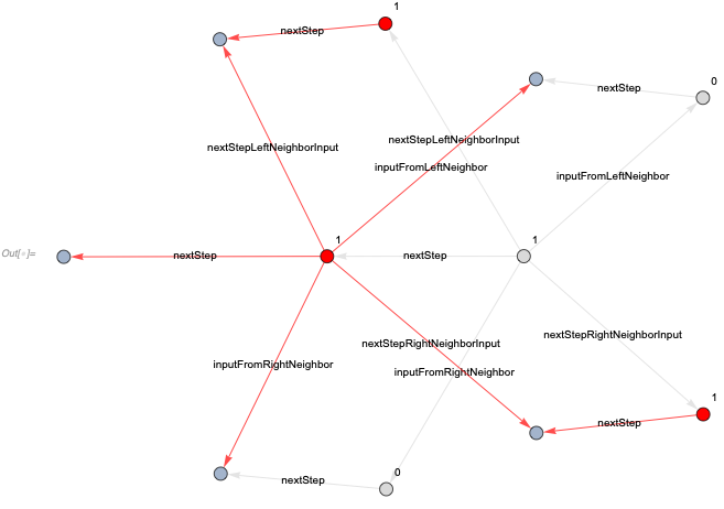
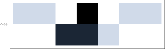
For an example where both neighbors are white, and the center is black, we get this step where old edges are in gray, and the new edges are in red
In[] := With[{states =
   SetReplace[Join[ ... (* CA cell blocks *)],
       caRules[110], #] /. { ...} & /@ {0, 1}},
 HighlightGraph[
  Graph[ ...] &[
   Union[Complement[states[[1]], states[[2]]],
    Complement[states[[2]], states[[1]]]]], {Style[
    Complement[states[[1]], states[[2]]], LightGray],
   Style[Complement[states[[2]], states[[1]]], Red]}]]
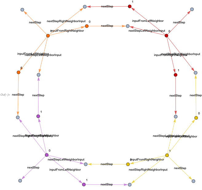
The entire graph after this step looks like this (with new edges highlighted in red), where one can see that the evolution of the same cell is blocked as there is no input from the neighbors
In[] := With[{states =
   SetReplace[Join[ ... (* CA cell blocks *)],
       caRules[110], #] /. { ...} & /@ {0, 1}},
 HighlightGraph[Graph[ ...] &[states[[2]]],
  Complement[states[[2]], states[[1]]]]]
We can confirm that this system does not overlap after running it for 10 steps
In[] := SetSubstitutionSystem[caRules[110], Join[ ... (* CA cell blocks *)],
  10, "CheckConfluence" -> True]["ConfluentQ"]
Out[] = Missing["Unknown"]
Missing is returned because the code only checks for overlaps between edges at the current step, but it is possible for overlaps to occur between space-like pair of events even if some of the vertices for one of them are already deleted. For this particular system, it is easy to see that this is not occurring, hence it is in fact confluent.
Localization
In the above, we simulated labeled edges and vertices by creating global vertices with names such as "inputFromLeftNeighbor", "nextStep", "1", and representing labeled edges by hyperedges passing through these global vertices, i.e.,
Labeled[x -> y, "nextStep"] <> {x, "nextStep", y}
However, it would be interesting to see if we can make the rules local, i.e., not involving any global vertices, and only depending on the vertices nearby the application site. This is indeed straightforward to do by making use of hyperedges with varying numbers of vertices, i.e.,
caLocalization = {
   {x_, "inputFromLeftNeighbor", y_} :> {x, x, y},
   {x_, "inputFromRightNeighbor", y_} :> {x, y, x},
   {x_, "nextStepLeftNeighborInput", y_} :> {x, x, x, y},
   {x_, "nextStepRightNeighborInput", y_} :> {x, x, y, x},
   {x_, "0"} :> {x},
   {x_, "1"} :> {x, x},
   {x_, "nextStep", y_} :> {x, y, y}
};
Now, we can localize both the rules and the initial condition to get the local evolution
In[] := SetSubstitutionSystem[caRules[110] /. caLocalization,
   Join[ ... (* CA cell blocks *)] /. caLocalization, 3] /@
  Range[0, 3] //
 GraphicsGrid[
   Partition[HypergraphPlot[#, ImageSize -> Scaled[1]] & /@ #, 2],
   ImageSize -> Scaled[1]] &
To decode it, one can look at the number of loops in the cell centers: 4 loops means 0, 5 loops means 1, so decoding evolution from above, we get {1,0,1,0}, {1,1,1,1}, {0,0,0,0}, {0,0,0,0}, which matches the evolution of the actual CA:
In[] := ArrayPlot[CellularAutomaton[110, {0, 1, 0, 1}, 3], ...]
We can demonstrate that this system is confluent as well
In[] := SetSubstitutionSystem[caRules[110] /. caLocalization,
  Join[ ... (* CA cell blocks *)] /. caLocalization, 10,
  "CheckConfluence" -> True]["ConfluentQ"]
Out[] = Missing["Unknown"]
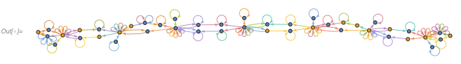
We can trivially extend this to any number of cells. For 10 cells, for instance, we get
In[] := SetSubstitutionSystem[caRules[110] /. caLocalization,
  Join @@ Table[
     caBlock[ToString[Mod[index, 10]],
      ToString /@ {Mod[index - 1, 10], Mod[index + 1, 10]},
      If[index == 1, 1, 0]], {index, 1, 10}] /. caLocalization, 8] //
 HypergraphPlot[#1[-1], ImageSize -> Scaled[1]] &
that maps to {1,1,0,1,0,1,1,1,1,1} after 8 steps, same as rule 110 CA
In[] := ArrayPlot[CellularAutomaton[110, {1, 0, 0, 0, 0, 0, 0, 0, 0, 0}, 8], ...]
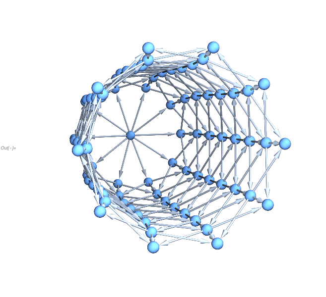
It is interesting to see how the causal network looks like in this case
In[] := SetSubstitutionSystem[ ...]["CausalNetwork"] // ... (* Graph3D *)
Infinite Grid
Proving universality however requires an infinite grid. We can achieve that by initially attaching the ends of the grid by specially labeled "left/right end" cells, and then adding new rules to expand these ends.
Specifically, we can construct the following four-cell structure where one of the end cells is colored in red, and the grid cell it is attached to is colored in yellow
In[] := Join[Catenate[{caBlock["0", {"leftEnd", "1"}, 0],
     caBlock["1", {"0", "2"}, 1], caBlock["2", {"1", "3"}, 0],
     caBlock["3", {"2", "rightEnd"},
      1]} /. {"rightNeighborInput[leftEnd]" -> "leftEnd",
     "leftNeighborInput[rightEnd]" -> "rightEnd"}], {{"leftEnd",
    "inputFromRightNeighbor", "leftNeighborInput[0]"}, {"leftEnd",
    "leftEnd"}, {"rightEnd", "inputFromLeftNeighbor",
    "rightNeighborInput[3]"}, {"rightEnd",
    "rightEnd"}}] // ... (* HighlightGraph *)
For the rule, we essentially need to replace the end cells with new white blocks connected to new ends, i.e.,
endExtensionRules = {{{xCenter_, "inputFromLeftNeighbor",
      leftEnd_}, {leftEnd_, "inputFromRightNeighbor",
      xLeftNeighborInput_}, {leftEnd_, "leftEnd"}} :>
    Module[{cellCenter, nextStepLeftNeighborInput,
      nextStepRightNeighborInput, nextStepCenter, newLeftEnd,
      leftNeighborInput, rightNeighborInput}, {
      {cellCenter, "nextStepLeftNeighborInput",
       nextStepLeftNeighborInput},
      {cellCenter, "nextStepRightNeighborInput",
       nextStepRightNeighborInput},
      {cellCenter, "nextStep", nextStepCenter},
      {cellCenter, "inputFromLeftNeighbor", newLeftEnd},
      {newLeftEnd, "leftEnd"},
      {newLeftEnd, "inputFromRightNeighbor", leftNeighborInput},
      {cellCenter, "inputFromRightNeighbor", xLeftNeighborInput},
      {cellCenter, "0"},
      {leftNeighborInput, "nextStep", nextStepLeftNeighborInput},
      {leftNeighborInput, "0"},
      {rightNeighborInput, "nextStep", nextStepRightNeighborInput},
      {rightNeighborInput, "0"},
      {xCenter, "inputFromLeftNeighbor", rightNeighborInput}
      }], ... (* left <-> right *)};
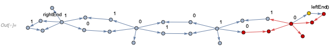
Running these rules from a single black cell will extend the edges indefinitely
In[] := SetSubstitutionSystem[endExtensionRules,
   Join[caBlock["0", {"leftEnd", "rightEnd"},
      1] /. {"rightNeighborInput[leftEnd]" -> "leftEnd",
      "leftNeighborInput[rightEnd]" -> "rightEnd"}, {{"leftEnd",
      "inputFromRightNeighbor", "leftNeighborInput[0]"}, {"leftEnd",
      "leftEnd"}, {"rightEnd", "inputFromLeftNeighbor",
      "rightNeighborInput[0]"}, {"rightEnd", "rightEnd"}}], 3] /@
  Range[0, 3] // ... (* Graph *)
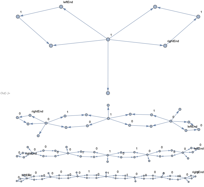
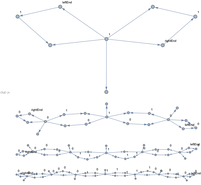
Combining the two sets of rules together, we can get evolution of the CA on an infinite grid
In[] := SetSubstitutionSystem[Join[endExtensionRules, caRules[110]],
   Join[caBlock["0", {"leftEnd", "rightEnd"},
      1] /. {"rightNeighborInput[leftEnd]" -> "leftEnd",
      "leftNeighborInput[rightEnd]" -> "rightEnd"}, {{"leftEnd",
      "inputFromRightNeighbor", "leftNeighborInput[0]"}, {"leftEnd",
      "leftEnd"}, {"rightEnd", "inputFromLeftNeighbor",
      "rightNeighborInput[0]"}, {"rightEnd", "rightEnd"}}], 3] /@
  Range[0, 3] // ... (* Graph *)
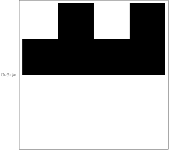
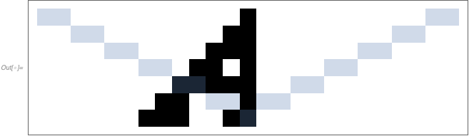
Note, the evolution does not happen row-by-row, but instead we get past cones, for instance after 3 steps, we get the cells highlighted in blue
In[] := CellularAutomaton[110, {{1}, 0}, {1, {-3, 3}}] // ... (* ArrayPlot *)
We can localize these rules similarly as before just adding new types of edges for left and right ends
caLocalizationInfinite = {
   {x_, "inputFromLeftNeighbor", y_} :> {x, x, y},
   {x_, "inputFromRightNeighbor", y_} :> {x, y, x},
   {x_, "nextStepLeftNeighborInput", y_} :> {x, x, x, y},
   {x_, "nextStepRightNeighborInput", y_} :> {x, x, y, x},
   {x_, "0"} :> {x},
   {x_, "1"} :> {x, x},
   {x_, "nextStep", y_} :> {x, y, y},
   {x_, "leftEnd"} :> {x, x, x, x, x},
   {x_, "rightEnd"} :> {x, x, x, x, x, x}
};
Running that for 3 steps, we then get
In[] := SetSubstitutionSystem[
   Join[endExtensionRules, caRules[110]] /.
    caLocalizationInfinite, ... (* initial condition *)/.
    caLocalizationInfinite, 3][-1] //
 HypergraphPlot[#, ImageSize -> Scaled[1]] &
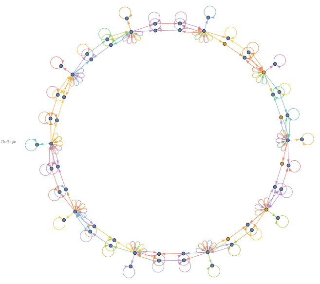
After 10 steps we get
In[] := SetSubstitutionSystem[
   Join[endExtensionRules, caRules[110]] /.
    caLocalizationInfinite, ... (* initial condition *)/.
    caLocalizationInfinite, 12][-1] //
 HypergraphPlot[#, ImageSize -> Scaled[1],
   GraphLayout -> "SpringEmbedding"] &
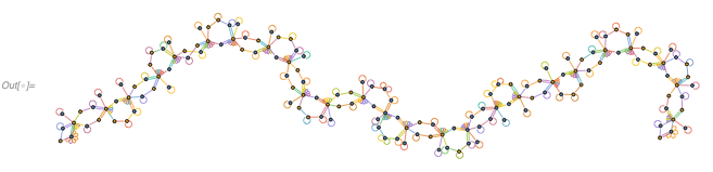
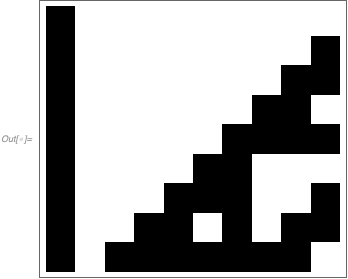
which corresponds to a slice of the CA
In[] := CellularAutomaton[110, {{1}, 0}, {6, {-12, 12}}] // ... (* ArrayPlot *)
Of course, by changing the order at which the rules are applied, any space- (including light-)like slice of the CA can be obtained.
Note, it is straightforward to extend this approach to produce periodic initial conditions as well, which is what's required for the proof of universality of rule 110.
We can finally show that this system is also confluent
In[] := SetSubstitutionSystem[
  Join[endExtensionRules, caRules[110]] /.
   caLocalizationInfinite, ... (* initial condition *)/.
   caLocalizationInfinite, 12,
  "CheckConfluence" -> True]["ConfluentQ"]
Out[] = Missing["Unknown"]
Thus we demonstrated that it is possible to construct a universal non-overlapping set substitution system.
Future Work
In the previous section we found a universal confluent set substitution system. However, that system is rather large. In fact, the total number of vertices references in the combination of the rules and the initial condition is
In[] := Length@Flatten[{ ... (* rules & initial condition *)} /.
   RuleDelayed -> List]
Out[] = 587
It would be interesting to see what is the smallest system possible that is both confluent and exhibits complex behavior.
Critical pair completion also requires more investigation, in particular, it would be interesting if known quantum effects such as entanglements, Bell's experiment, and double-slit experiment can be reproduced with this set up.
 Attachments:


