Overview
Everyone has different ideas about what a Quantum Cellular Automaton (QCA) should do. In my opinion, a QCA takes in a quantum state and evolves it using quantum operations that are dependent on its neighbours. This is analogous to the classical CA where classical states (0 or 1) are evolved using classical operations dependent on their neighbours. We define two types of QCA models that could be used to explore. We also show several applications to physics by slightly modifying the QCA model. The first model is based on the quantum teleportation protocol, the second is evolving a tensor product. However, there were many failed models before these two that I will talk about as well. QCAs can also be applied to physical systems. Applications in physics include showing the evolution of a quantum state (includes simulating a CNOT gate), showing a coupled two-state system, showing precession of a two state system in a magnetic field, and showing a simple (NN) Heisenberg spin chain.
?QCA Teleportation Model
This model starts with a list of two state systems (qubits).
$$ \alpha _1\text{ $|$0$> $+}\beta _1\text{$|$1$> $,}\alpha _2\text{$|$0$> $+}\beta _2\text{$|$1$> $,...} $$
The nearest neighbour of a given qubit is "teleported" to the next state using the quantum teleportation protocol. First, a [CapitalPhi]^+ bell state is introduced. The [CapitalPhi]^+ state is then combined with the nearest neighbour qubit, creating a quantum system with 3 qubits. Periodic boundary conditions are applied. The nearest neighbour qubit and one of the entangled qubits in the system is put through a CNOT gate, effectively entangling the two. Then the nearest neighbour qubit is put through a Hadamard gate to ensure both exist in the same basis. Then both (nearest neighbour and one of the entangled) are measured using any arbitrary measurement, here I used measurement in [Sigma]^x basis. Depending on the measurement obtained above, the nearest neighbour qubit is teleported by transforming the third entangled qubit, allowing us to perform further operations on it later. Also, based on the measurement an operation is chosen for the j^th qubit. There are four possible outcomes: 00, 01, 10, 11. A list of operators is defined. One of the operators is then applied based on the measurement applied. Operators can be any combination of four matrices, a possible combination is to use PauliX, PauliY, PauliZ, and Hadamard. The function is mapped across the entire list of qubits, and a new state is created. The state is then evolved several times, depending on the number of steps (n). This gives a list of states very much like a CA.
To visualize these states, I created some type of RGB scheme. Here is what four of the states look like.
?
The rest are combinations of these colours. Finally the QuantumCellularAutomataTeleport function can be created.
QuantumCellularAutomataTeleport[{operatorHadamard, operatorPauliX, operatorPauliY, operatorPauliZ}, 50]
?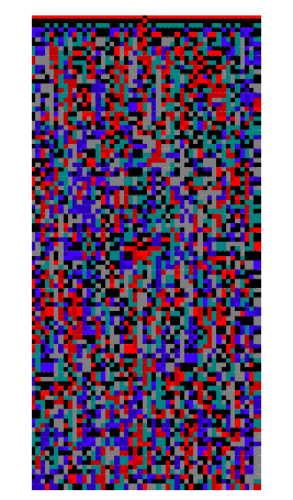
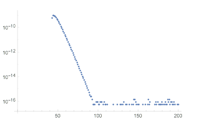
The result looks random, but actually isn't, as told by a randomness tester. The test it failed is the run length test. This could mean that there is unusual clustering of similar states, which is something we can sort of see in the picture. It would be interesting to explore why this happens.
Quantum Cellular Automata Tensor Model
Another model for the QCA includes evolving an entire state together instead of separate qubits individually. This would be analogous to having some sort of spin chain system. A state of N qubits is taken. I will let N = 3.
$$ c_1\text{ $|$000$> $+}c_2\text{$|$001$> $+}c_3\text{$|$010$> $+}c_4\text{$|$011$> $+}c_5\text{$|$100$> $+}c_6\text{$|$101$> $+}c_7\text{$|$110$> $+}c_8\text{$|$111$> $} $$
The state vector of this is the coefficients c1
c8.
The way this model would work is by applying a composition of operations applied on a qubit and its neighbour. There are N qubits and k is the number of operators.
For j in range {1,...,N} compute the operator for the jth qubit by the following, apply it to the jth qubit. Do this for all j in N, then add all the resulting states.
$$\left(\sum _{j=1}^N u^{k-1}{}_j u^{k-1}{}_{j+1} u^k{}_j u^k{}_{j+1}\text{...}u_j u_{j+1}\right)$$
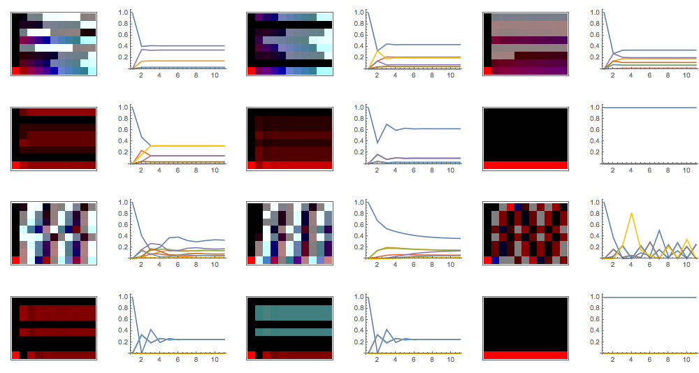
Now, instead of choosing from a list of operators we are composing a list of operators and applying them repeatedly. An interesting thing to examine about this type of QCA is the probability of being in a given state. This would be the norm of the coefficient of each possible state squared. Plotting several of these along with their corresponding QCAs leads to this.

When I show these results to physicists, it makes sense. They talk about an "equilibrium" state that the system reaches or of an oscillating equilibrium state (like that produced SqrtNOT). However, from a linear algebra perspective this is not immediately obvious. How can applying any arbitrary combination of operators onto any initial vector result in period behaviour? Not even periodic, but result in probabilities of being in each state that are constant for most of the time. However, the physics behind this makes sense.
The relationship between the computational complexity of the inverse operation (the operation that will go from the equilibrium state to the initial state) and the time it takes for the system to reach equilibrium could potentially have a significant relationship. However, the effect we see here is analogous to thermalization. Plotting the norms of a given state against time gives a plot that shows behaviour analogous to thermalization. This can be further analyzed for different types of states.
Physical Systems
This model can also be applied to physical systems. This includes the evolution of a two-state system, as well as precession in a magnetic field.
I took a two level system Hamiltonian, and created an operator that would time evolve it. The time evolution operator depends on the coupling constant (t) and epsilon, I took different values for each and displayed the results using a QCA.
showQubitEvolution[operatorTime, onequbit, matrixHamiltonian]
?
$epsilon = 2;
matrixHamiltonian = {{$epsilon,$t},{$t,-$epsilon}};
?
$t = 0.5;
matrixHamiltonian = {{$epsilon,$t},{$t,-$epsilon}};

Failed Models
There were several models that failed as well. I have them in my gitHub, but here is an explanation for one of them.
This model formulates QCAs using a two qubits per cell system. Each time step has an interaction step followed by an evaluation step. Each cell has a "state" qubit and a "control" qubit. First, the state qubit on the right is composed with the control qubit in the middle using some operator (e.g. CNOT) and the control qubit is partial traced out. Then, that control qubit is composed with the state qubit on the left using some operator and partial traced out again. This is the end of the interaction step. Now, we take the state qubit of the middle cell and the new control qubit and compose them using some operator (e.g.. Fourier) to get the new cell, this is the evaluation step. This is then repeated for all cells in the row. The arrows represent partial traces, and lines represent operations.
?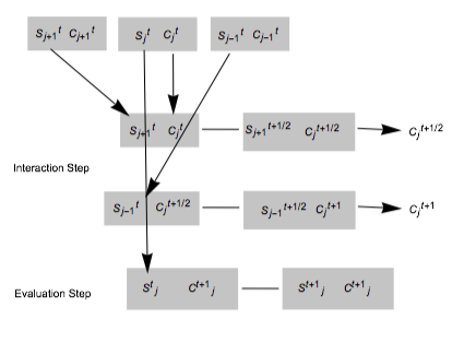
The issue arisen with this model was the inability to apply a quantum partial trace to the control qubit after it had been in an impure state with the state qubit. So the evolution only worked for simple quantum gates that did not produce any sort of real interaction between the state and control qubit, which is the whole point of a QCA. However, if this could be done without taking a partial trace of the qubits, this model is still possible.
Future Works
For the future, a definite relationship between the time taken to evolve into an equilibrium state and the computational complexity of the evolution of the state into the equilibrium state. It would also be useful to explore more rules and gather data to explore the relationship further. There were also a couple of failed models that should be revisited and attempts could be made to implement them. It is also possible to explore further physics applications including simulating NMR and more complicated Heisenberg spin chains.
GitHub Repo