Abstract
Determine how good a PC is in a universal score is always handy when it comes to comparing to other machines. Nowadays, with each kind of focus on hardware design, it's hard to say one machine will always out-perform the other just based on the model. Therefore, benchmarking, testing the machine performance, to determine how good it is in a certain kind of workload is necessary.
Introduction
In this project, benchmarking one's machine under WL environment to see which machine perform the best is the main focus. The whole benchmarking will be separated into 4 main parts, while each section will include testing the following:
- CPU
- Both single and multicore (parallel) performance
- Disk
- RAM
- Both speed and the total amount of RAM in one's machine
- GPU
- Only Nvidia GPU was available, CUDA only, no OpenCL testing available for AMD
After running the specific test for each part of the hardware, the calculation time will be recorded and transform into points instead. All the testing level has been set so the calculation time will be around 3~10 seconds on the machine coded this project due to limited testing time.
Following is the (Calculation time vs Points) formula and its plot:
$$900-900 \tan ^{-1}(0.02 t)$$
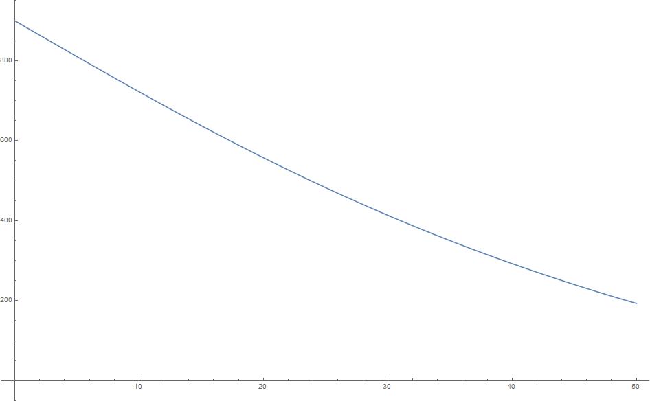
Notice that the transform formula from time to points isn't linear; the potential issue will be hard to tell the difference in terms of performance. But the advantage of using this formula is the tester will know exactly above what score the machine is considered "well above average," and as the points increases, the value of each point increases as well.
It's like the famous college entrance test, SAT, improving from 750 to 800 is always harder than from 600 to 700.
Benchmarking
CPU
Since the default function won't be using parallelism, it's highly favoring single-core frequency than multi-core low frequency, so the result will be similar to testing a video game. During the testing, if the parallel function is available, this test will check both (Do for example) ParallelDo and Do and weighted the score of 7:3 as this will give multi-core more credit than they should've gotten as well as letting the user know they should use Parallel function whenever it's available.
The CPU test set will be including the following:
- Finding PI
- Finding Prime number (Parallel available)
- Compile Time
- Finding Eigenvalues (Parallel available)
- LinearSlove (Parallel available)
- Transpose
- Random number sorting (Parallel available)
- SphericalPlot3D (monitored on GPU-Z, this is rendered by CPU)
- NSlove (Parallel available)
Cellular 3D
Cell3DTime = RepeatedTiming[Graphics3D[Cuboid/@Position[#,1],
             ImageSize->Full]&/@CellularAutomaton[
             {30, {2, 1}, {2, 2,2}},{{{{1}}},0},30];][[1]];
RAM
This task is mainly for testing RAM, both speed and the total amount of RAM on one's machine.
In real life application, the performance impacted by RAM speed is very insignificant; instead, the total amount of RAM available to use is usually the main focus.
Therefore, this test set will factor in both speed and amount; the speed score will be around 200~300 while the score for the amount of RAM will be around 1500+.
Following is the test set used to test RAM, filling 4 different sizes of arrays with 0s and find its slope and then plot it in time vs. byte.
Notice the unit is not the standard unit for RAM, MHz, instead, it's in MB/sec. However, since it will be converted to points eventually with the speed of RAM in MB/sec divided by 10 (lowering down the significance to a reasonable point)
RAMSpeedTest[] := Module[{
AA,A,B,CC,AASize={2000,2000},ASize={5000,5000},
BSize={10000,10000},CCSize={15000,15000},Speed,Time,Score
},
Speed=UnitConvert[Quantity[
D[Fit[{
{RepeatedTiming[AA=ConstantArray[0.,AASize]][[1]],ByteCount[AA]},
{RepeatedTiming[A=ConstantArray[0.,ASize]][[1]],ByteCount[A]},
{RepeatedTiming[B=ConstantArray[0.,BSize]][[1]],ByteCount[B]},
{RepeatedTiming[CC=ConstantArray[0.,CCSize]][[1]],ByteCount[CC]}},
{1,x},x],x],
"Bytes"/"Seconds"],"Megabytes"/"Seconds"];

ClearAll[A,B,CC,AA];
Score=QuantityMagnitude[Speed]/10;
<|"RAMSpeed" -> Speed,"RAMScore" -> Score|>
]
The amound of RAM is found by:
RAMMuch[]:=
Module[{Weight=350,HowMuch,Score},
Score=Weight*Sqrt[
QuantityMagnitude[HowMuch=SystemInformation["Machine","PhysicalTotal"]]]
;
<|"RAMScore" -> Score,"RAMTotal" -> HowMuch|>
]
While the score is calculated by: $$350 \sqrt{\text{Total} \text{} \text{ RAM (in GB) }}$$
Disk
This part is for disk benchmarking, disk speed is usually considered more important than RAM speed (but slower of course) in terms of performance, and often the amount of disk available isn't an issue since it's hard to have one program export a 100+ GB file, the situation is reverse compared to RAM.
Although, the speed got from the below test doesn't really agree (either sequential or random) on a real disk benchmarking (CrystalDiskMark 6) software, but it indeed is testing disk speed so just see it as "apparent speed" instead and convert it to points, as long as it scales as the real speed increases, this score should still be meaningful.
Following is the method used to test disk speed:
DiskSpeed[] := Module[
    {
    strLength = 500000000, str, testfile,
    diskwritetime, diskreadtime, diskwritespeed,
    diskreadspeed
    }
    ,
    str = StringJoin[ConstantArray["0", strLength]];
    testfile = CreateFile[];
    diskwritetime = First@AbsoluteTiming[WriteString[testfile, str]];
    diskreadtime = First@RepeatedTiming[ReadString[testfile]];

    diskwritespeed = UnitConvert[
       Quantity[ByteCount[str]/diskwritetime, "Bytes"/"Seconds"],
       "Megabytes"/"Seconds"
       ];
    diskreadspeed = UnitConvert[
       Quantity[ByteCount[str]/diskreadtime, "Bytes"/"Seconds"],
       "Megabytes"/"Seconds"
       ];

    <|"ApparentDiskWriteSpeed" -> diskwritespeed, "ApparentDiskReadSpeed" -> diskreadspeed|>
]
Disk score is calculated with the following: $$ \text{Apparent Write Speed} + \text{Apparent Read Speed }$$
GPU
GPU isn't being used in normal functions in WL environment besides training the neural network. But it is a big part of the PC, and as the usage of training neural network increases, GPU will play a huge role. Since the machine coded this project supports CUDA (RTX 2070 max-Q) but not OpenCL, this project will be testing CUDA functions instead and give a reasonable estimate for GPU performance.
The test set includes CUDADot, CUDATranspose, NetTrain for dot operation, convolution and image training from example data. Following are 2 out of total 5 tests, convolution training, and dot training:
nettest=NetChain[{100,BatchNormalizationLayer[],Ramp,
    300,BatchNormalizationLayer[],Ramp,300,Ramp,45,Ramp,90},
    "Input"->{80,80}];
convNet=NetChain[{ConvolutionLayer[16,3],
    BatchNormalizationLayer[],Ramp,ConvolutionLayer[32,3],
    BatchNormalizationLayer[],Ramp,ConvolutionLayer[64,3],
    BatchNormalizationLayer[],Ramp,ConvolutionLayer[17,3],
    AggregationLayer[Max]},"Input"->{80,80}];
dottrainingData=<|"Input"->RandomReal[1,{1000,80,80}],
    "Output"->RandomReal[{-20,20},{1000,90}]|>;
{dottraintime,dottrained}=RepeatedTiming@NetTrain[nettest,dottrainingData,
    TargetDevice->"GPU",MaxTrainingRounds->120,
    TrainingProgressReporting->None];
convtrainingData=<|"Input"->RandomReal[1,{1000,80,80}],
    "Output"->RandomReal[{-20,20},{1000,17}]|>;
{convtime,convtrained}=RepeatedTiming@NetTrain[convNet,convtrainingData,
    TargetDevice->"GPU",MaxTrainingRounds->120,
    TrainingProgressReporting->None];
For the scoring system, GPU will be using the same formula as CPU.
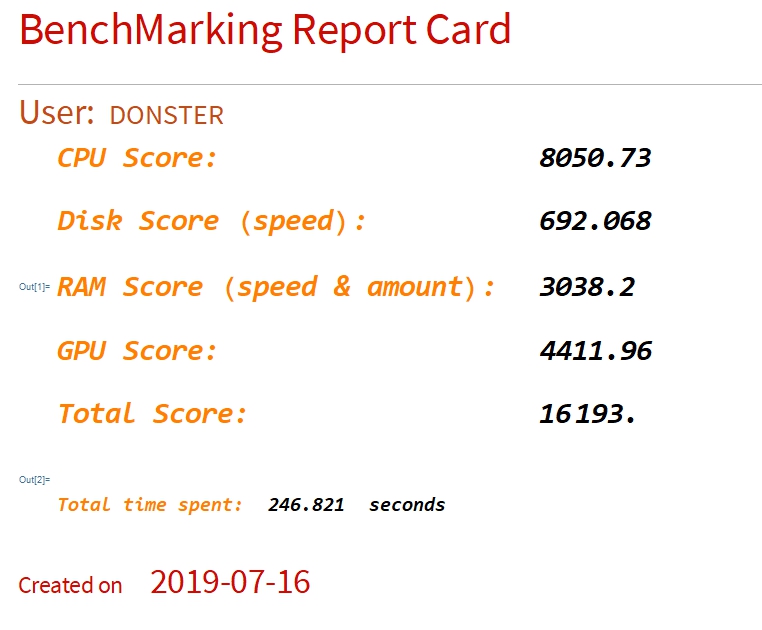
Result
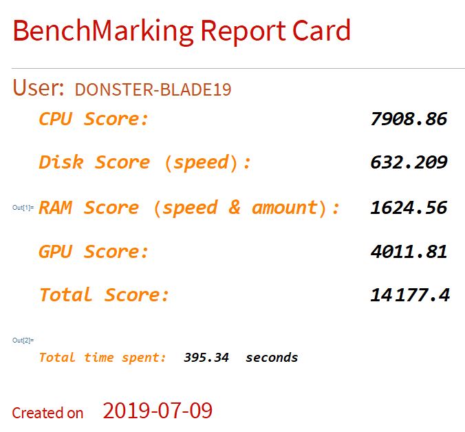
After testing, a report card, including all 4 test sets score, total score, machine name, and total time spent, will be generated. Here are a few examples, including specification, obtained manually.
- Machine name: DONSTER-BLADE19
- CPU: Intel Core i7 9750H @ 2.60 GHz
- GPU: Nvidia RTX 2070 with Max-Q
- RAM: 16 GB @ 2667 MHz
- Disk: Samsung PM 981
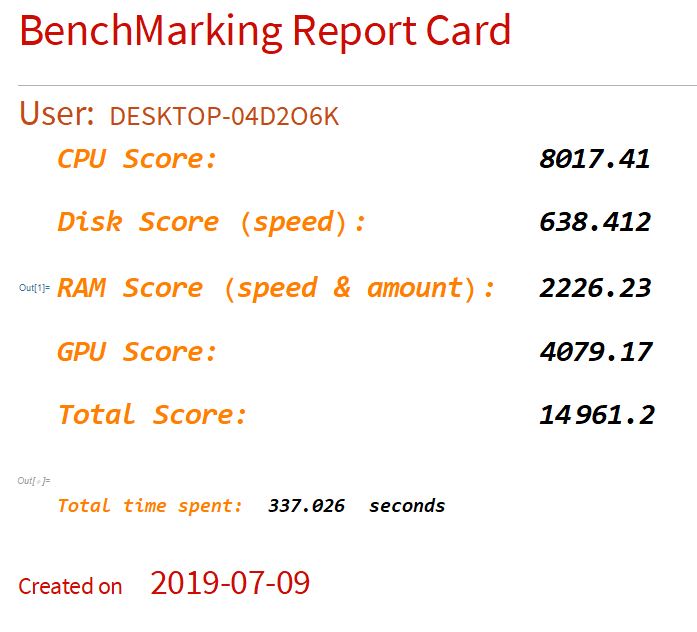
- Machine name: DESKTOP - 04D2O6K (as known as The GPU Machine)
- CPU: Intel core i7 7700 @ 3.60 GHz
- GPU: Nvidia GTX 1080 TI FE
- RAM: 32 GB @ 2400 MHz
- Disk: Intel 660p
- Machine name: Donster (writer's personal rig)
- CPU: Intel core i7 8700K OC@ 5.20 GHz AVX -2
- GPU: EVGA GeForce RTX 2080 Ti FTW3 Ultra Gaming @ 2070 MHz
- RAM: 64 GB @ 3600 MHz
- Disk: Intel Optane SSD 900P 480GB
Conclusion
After running the whole benchmark, the tester can obtain a report card that includes all the relevant information needed to compare to other machines. Compare to the current benchmarking built-in suite in Mathematica, this benchmarking suite tested much more aspects and includes benchmarking GPU, which is relevant hardware when it comes to machine learning.
Future Work / Improvement
- Improve the algorithm of calculating points
- More testing sample
- Increase the GPU and CPU testing level to differentiate high-end components
- Loading bar for the whole benchmark process
- Run GPU with CUDA code to find prime numbers or some large integer calculation
- An OpenCL version for AMD GPU user
- Obtain necessary system information such as GPU/CPU model, clock speed...etc.
- Ranking system
 Attachments:


