Introduction
Discrete plots are one of the charts that are used widely in almost all fields of science, business and industry for data virtualization. It is often of great interest to extract numerical values of data from discrete plots in the form of images for further analyzing and processing. However, most data extraction software requires manual data extraction and axes establishment from the user which is time-consuming. In this project, we present an automated data extraction system for discrete plot images that utilizes a semantic segmentation approach where image pixels are classified as being different parts of the image by modifying a neural network model called ResNet-22.
Methods
The project consists of three parts: 1) generating training and testing data, 2) pixel classification and 3) data extraction. To achieve as much diversity as possible for the training data, we randomize the axes ranges and scales, data point colors and data point shapes for a large amount of data. We then use a semantic segmentation approach to identify and classify pixels in an image that correspond to four distinct parts of it: background, axes, axes labels and data points. Finally, we use an imaging processing approach to extract numerical coordinates of the data from discrete plot images.
Semantic segmentation (Pixel classification)
Dataset generation
The code below generates a set of training and testing data with a diverse range of color, axes ranges and data point shapes. Each generated data has a form of input -> output where the original image as being input and a tensor whose elements have values {1, 2, 3, 4} as being the output. Here the set {1, 2, 3, 4} represents the four distinct pixel classifications of the plot image as background, axes, axes labels and data points respectively. 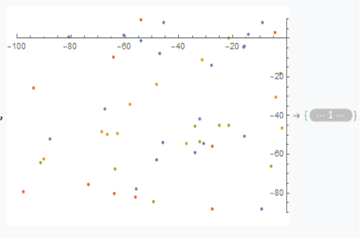
Neural net output segmentation tensor generation:
(* defining plot theme*)
theme = "default";
(* generating ranges for horizontal and vertical axes *)
ranges[ max_Integer, di_Integer ] := Flatten[Table[
   { { -100 + i, 0 + i }, { -100 + j, 0 + j } },{ i, 0, 100, 10 },{ j, 0, max, di } ],
    1 ]
(* generating random 2D points with five different colors for the plots *)
getRandomPointsList[ nPoints_Integer, ranges_ ] := ParallelMap[ Partition[ Transpose@{ RandomReal[ First[ # ], nPoints ], RandomReal[ Last[ # ], nPoints ] }, Round[ nPoints/5]]&, ranges ]
(* generating corresponding scattered plot images *)
getRasterizedPlots[ data_, ranges_ ] := ParallelMap[ Rasterize[ ListPlot[ First[ # ], PlotRange -> Last[ # ],PlotTheme -> theme ], ImageSize -> { 360, 240} ] &, Transpose[ { data, ranges } ] ]
(* extracting raw axes from scattered plots *)
getRawAxes[ data_, ranges_ ] :=
  ParallelMap[
   AlphaChannel[
    Rasterize[
     ListPlot[ First[ # ], PlotRange -> Last[ # ], PlotStyle -> Transparent, LabelStyle -> Transparent, BaseStyle -> { Antialiasing -> False }, PlotTheme -> theme ],
     Background -> None, ImageSize -> { 360, 240 } ] ]&, Transpose[ { data, ranges} ]
             ]
(* extracting raw labels from scattered plots *)
getRawLabels[data_,axes_,ranges_] :=
  MapThread[
   ImageDifference[
    Binarize[
     AlphaChannel[
      Rasterize[
       ListPlot[#1, PlotRange-> #3, PlotStyle->Transparent, BaseStyle->{Antialiasing->False},PlotTheme->theme],
               Background->None, ImageSize->{360,240}]], 0],#2]&, {data, axes, ranges}
           ]
(* generating binarized points from scattered plots *)
getBinarizedPoints[data_,ranges_]:=
  ParallelMap[
   AlphaChannel[
    Rasterize[
     ListPlot[First[#], PlotRange->Last[#], AxesStyle->Transparent, BaseStyle->{Antialiasing->False},PlotTheme->theme], Background->None, ImageSize->{360,240}]]&,
         Transpose[{data,ranges}]
             ]
(* filtering out points that are overlapping with the axes and axes labels *)
getAxes[axes_, binarizedPoints_]:= MapThread[ImageSubtract[#1, #2]&,{axes, binarizedPoints}]
getLabels[binarizedPoints_, labels_]:= MapThread[ImageSubtract[#1, #2]&,{labels, binarizedPoints}]
(* generating backgrounds from scattered plots *)
getBackgrounds[axes_,labels_,binarizedPoints_]:= MapThread[ColorNegate[ImageAdd[#1,#2,#3]]&,{axes,labels,binarizedPoints}]
(* generating image segmentation tensors from scattered plots with four classes where background, axes, axes labels and data points are labeled as 1, 2, 3, 4 respectively *)
segmentateImage[background_,axes_,labels_,binarizedPoints_]:= Round[ImageData[ImageAdd@@MapThread[ImageMultiply,{Image[{background, axes, labels, binarizedPoints},"Real32"],{1,2,3,4}}]]]
getSegmentations[dataPoints_,ranges_]:=Module[{r=ranges,data=dataPoints, binarizedPoints, axes, labels, backgrounds},
binarizedPoints=getBinarizedPoints[data,r];
axes=getAxes[getRawAxes[data,r], binarizedPoints];
labels=getLabels[binarizedPoints, getRawLabels[data, axes,r]];
backgrounds=getBackgrounds[axes, labels, binarizedPoints];
MapThread[segmentateImage[#1, #2, #3, #4]&,{backgrounds, axes, labels, binarizedPoints}]
]
Generate a mixture of "monochrome" and "default" themes dataset:
(* generating training data where scattered plots are used as inputs and image segmentation is used as outputs for the NetTrain function *)
createTrainingData[ max_, di_, nPoints_Integer ] := Module[{ranges=ranges[max,di], data, plotsImages, segmentations},
data = getRandomPointsList[ nPoints, ranges ];
plotsImages = getRasterizedPlots[ data, ranges ];
segmentations = getSegmentations[ data, ranges ];
MapThread[ Rule[ #1, #2 ]&, { plotsImages, segmentations } ]
]
(* create a dataset with "default" theme *)
 defaultThemePlots = Flatten@Table[ createTrainingData[ 100, 10, 50 ], 5 ];
(* create a dataset with "monochrome" theme *)
 monochromeThemePlots = Flatten@Table[createTrainingData[100,10,50],5];
(* create a mixed dataset with both "default" and "monochrome" themes by joining the above
datasets *)
SeedRandom[1234];
data = RandomSample[ Join[ monochromeThemePlots, defaultThemePlots ] ];
Generate and export training and testing data:
(* set working directory *)
SetDirectory[NotebookDirectory[]]
(* export generated data to working directory *)
Export["data_diversified.wl",data]
(* create training and testing dataset *)
trainingSet=Take[data,1100];
testSet=Take[data,-110];
Import and modify the ResNet-22 net
(* import the ResNet-22 neural network from the Wolfram Neural Net Repository *)
net = NetModel[ "Dilated ResNet-22 Trained on Cityscapes Data"]
(* modify the ResNet-22 neural network to meet the input needs *)
ourNet = NetReplacePart[ net, {"input_0" -> NetEncoder[ { "Image" , { 360, 240 } } ], "Output" ->
NetDecoder[ { "Class", Range[ 1,19 ], "InputDepth" -> 3 } ] } ];
Train the modified ResNet-22 net with GPU
(* train the modified neural network with generated training set using GPU *)
trainedNet = NetTrain[ ourNet, <|"input_0" -> First/@trainingSet, "Output" -> Last/@trainingSet|>, LossFunction -> CrossEntropyLossLayer[ "Index" ], TargetDevice -> " GPU " ]
Export trained net and generate net outputs
(* export trained neural network to local directory *)
Export["trained_net.wlnet",trainedNet]
(* import trained neural network *)
trainedNet = Import[ "trained_net.wlnet" ]
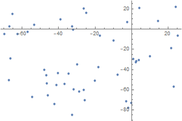
Apply the trained net, we obtain a tensor representation of the original discrete plot image with a colorized virtualization:
(* apply the trained neural network to the above input plot *)
trainedNet[ImageResize[input0, {360, 240}]] // Colorize
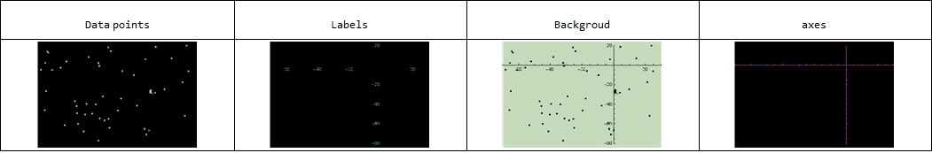
By setting other net output tensor elements to 0, we have the image segmentation:
(* get image segmentations *)
{pointsData, imageLabels, imageBackground, imageAxes} = {m/.{1->0,2->0,3->0}//Colorize, m/.{1->0,2->0,4->0}//Colorize, m/.{4->0,2->0,3->0}//Colorize, m/.{1->0,4->0,3->0}//Colorize}
Data extraction
To extract numerical coordinate values, we first extracted pixel positions for each data points and identified axes scales as image corners in order to obtain axes scale. For this project, we manually extracted axes label values which could be identified by optical character recognition (OCR) in future's work.
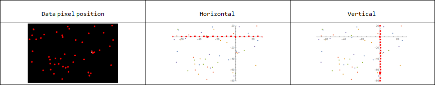
Extract data pixel position and axis scales
(* get pixel positions for the centers of data points *)
points = ComponentMeasurements[pointsData, "Centroid"][[All, 2]]
HighlightImage[pointsData,points]
In order to obtain axes scale, first identify axes lines and get clean image corners of them by constraining the distance between corner points and corresponding axes:
(* identify horizontal axes scales by treating them as image corners *)
dotOnX=SortBy[Select[ImageCorners[imageAxes, Method->"HarmonicMean"], RegionDistance[xAxis, #]<3 &],First];
HighlightImage[input0, dotOnX]
(* identify vertical axes scales by treating them as image corners *)
dotOnY=SortBy[Select[ImageCorners[imageAxes, Method->"HarmonicMean"], RegionDistance[yAxis, #]<3 &], Last];
HighlightImage[input0, dotOnY]
Next, calculate the average of the axes corner points to obtain the axis scales for both axes,
(* get vertical axis sclae by averaging the distances between ajacent corner points as shown above *)
ySteps=Sort[Differences[Last /@ dotOnY]];
ySteps=Drop[ySteps, FirstPosition[ySteps,Max[ySteps]]];
ySteps=Drop[ySteps, FirstPosition[ySteps,Max[ySteps]]];
ySteps=Drop[ySteps, FirstPosition[ySteps,Min[ySteps]]];
ySteps=Drop[ySteps, FirstPosition[ySteps,Min[ySteps]]];
yStep = Mean[ySteps]
(* get honrizontal axis sclae by averaging the distances between ajacent corner points as shown above *)
xSteps=Sort[Differences[First /@ dotOnX]];
xSteps=Drop[xSteps, FirstPosition[xSteps,Max[xSteps]]];
xSteps=Drop[xSteps, FirstPosition[xSteps,Min[xSteps]]];
xSteps=Drop[xSteps, FirstPosition[xSteps,Max[xSteps]]];
xSteps=Drop[xSteps, FirstPosition[xSteps,Min[xSteps]]];
xStep = Mean[xSteps]
as well as the origin:
(* get pixel position for the intersection between horizontal and vertical axes or the origin *)
originPoint = RegionIntersection[xAxis,yAxis]
By manually identifying axes labels, we are then able to convert data points pixel positions to coordinates in Cartesion systems:
(* convert pixel positions to coordinates in Cartesian system *)
listCoordinates = Function[p, {( First[p] - originPoint[ [1, 1, 1] ] )/xStep/4*20, (Last[p] - originPoint[ [1, 1, 2] ])/yStep/4*20}]/@points;
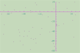
(* recover discrete data points *)
ListPlot[listCoordinates]
Extract data point color
To obtain color information, we use the original input image as reference and classify different colors:
(* label each pixel points in order *)
listPixelCoordinates = MapThread[Rule[#1,#2]&, {Range[49], points}];
(* identify the color for each pixel point by comparing to the original input image *)
listpointsColors = MapIndexed[RGBColor@PixelValue[ originalplot, #1 ] -> First@#2&,
Values@listPixelCoordinates]
(* classify data points by color *)
FindClusters[listpointsColors,6]
(* Recover data points color *)
result0 = ListPlot@Map[Part[listCoordinates,#]&,FindClusters[listpointsColors,6]]//Rasterize
We can then recover the input image: 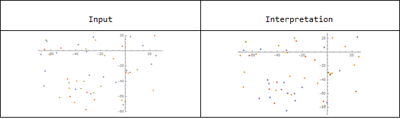
Conclusion and future work
The above pixel classification and image processing approach successfully recovered data points as numerical values from an image. Though the color identification is not robust enough for this case, it could be improved by finding the appropriate numbers of color groups. Furthermore, this method has difficulty identifying points that are clustered closely together or overlapped. As mentioned above, optical character recognition (OCR) can be applied for identifying axes labels to increase the system's automation level.
References
$[1]$ https://resources.wolframcloud.com/NeuralNetRepository/resources/Dilated-ResNet-22-Trained-on-Cityscapes-Data
 Attachments:


