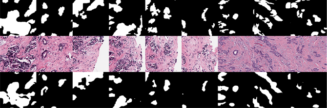
Fig. 1 portrays the images associated with a classic segmentation task, in this instance of so-called epithelium cells. The images in the upper row represent the masks rendered by professional, human pathologists; the middle row the original histopathological image; and the bottom row the images generated by the trained network. Each column represents all images associated with a single histopathological slide.

Background

Histopathological examination, the study of biopsied tissues and cells using microscopy, is one of the key means by which a wide range of illnesses are diagnosed across the world. However, the time, labor, and expertise required to perform these diagnostic processes, coupled with a deficit of trained pathologists, is driving a global trend of delayed or omitted histopathology services - potentially life-saving insights are not adequately reaching patients' care teams.

These challenges have elevated digital pathology, the machine-aided processing of digitized histopathology samples, to be a critical frontier of modern medical research. One of digital pathology's most pertinent tasks is that of automatic image segmentation: the delineation of specified tissue-, cell-, and organelle-level entities. Current segmentation models are largely based on hand-crafted algorithms. These algorithms require extensive, advanced feature engineering; profound expertise in pathology and machine learning to develop, maintain, and use; and, in addition, are typically only capable of segmenting a single type of entity. All of these factors contribute to these models being infeasible to deployment in clinical settings.

Thus, the aim of this little foray is to develop a deep neural network model that is capable of performing segmentation of tissue-, cell-, and organelle-level entities without relying on hand-crafted features.

General Method

To achieve the above aim we will explore the potential of the deep neural network Ademxapp Model A1, pre-trained on Cityscapes Data, to perform image segmentation on single types of cellular entities without relying on advanced, handcrafted features. As its name suggests, this particular Ademxapp model has previously been used to segment images of driving scenarios into nineteen semantic component classes (such as "road", "trees", and so on), achieving 80.6% mean IoU accuracy.

This pre-trained model will be applied to pre-existing, publicly available histopathology datasets, each dataset containing two sets of images: an original histopathological image, and a so-called "mask": an outline of a specified cell entity made by a professional pathologist (see figure 2). For this part of the investigation, we will train copies of the Ademxapp model to segment only one particular cellular entity at a time. The first Ademxapp copy will learn to segment nuclei, an organelle found within cells; the second Ademxapp copy will learn to segment tubules, which are large-scale tubular and fistular structures composed of cells; and finally, the third Ademxapp copy will learn to segment epithelium cells, which are a particular type of cells. As such, we will hopefully determine the potential for Ademxapp to be used as a segmentation network for histopathological entities across multiple several scales: the tissue-, cell-, and organelle-level.

However, for reasons of space, this blog post will only explicitly feature our investigation into the first Ademxapp's ability to segment nuclei.

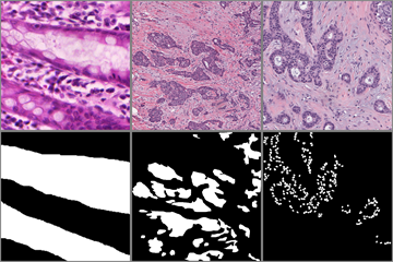
Fig. 2: An example of original histopathology images (upper row) and their respective corresponding masks (lower row). From left to right, the first column depicts tubules, the second column depicts epithelium cells, and the third column depicts nuclei

Task 1: Nuclei

Background

Nuclei typically exhibit marked changes when afflicted by various cancers. In particular, for multiple cancers, including estrogen receptive breast cancer, nuclear configuration and morphology is strongly correlated with disease progression and survival rates. Alike tubules and epithelium cells, nuclei thus form a crucial basis of multiple cancer grading schemes. An algorithm capable of rapid and reliable nuclear segmentation would therefore be a useful tool in making diagnostics more efficient, while decreasing inter- and intra-reader variance in critical metrics of epithelium area, stratification, and distribution.

Method

The nuclei dataset we will be using is a publicly available collection of 143 {2000, 2000} estrogen receptor positive breast cancer (ER+ BCa) images scanned at a magnification of 40x, each alongside its respective associated mask. Each mask was manually annotated by an expert pathologist. The investigation's pre-processing included up-sampling these images to {2048, 2048} before partitioning them into non-overlapping {256, 256} patches.

The patches were divided into training, testing, and validation sets in an 80:10:10 ratio. The training set patches were then used to fine-tune Ademxapp A1 pre-trained on Cityscape data. The code used an ADAM optimizer and ran for 20 rounds with a batchsize of 12 (11840 batches total).

Network Training Script

netModel = NetModel["Ademxapp Model A1 Trained on Cityscapes Data"];
netModel256 = 
  NetReplacePart[netModel, 
   "Input" -> NetEncoder[{"Image", {256, 256}}]];
firstPartNet = NetDrop[netModel256, -3];
finalNet = 
  NetJoin[firstPartNet, 
   NetChain@<|
     "linear2" -> 
      ConvolutionLayer[2, {3, 3}, "Stride" -> {1, 1}, 
       "PaddingSize" -> {12, 12}, "Dilation" -> {12, 12}], 
     "resize" -> ResizeLayer[{256, 256}], 
     "softmax/1" -> TransposeLayer[{1 <-> 3, 1 <-> 2}], 
     "softmax/2" -> SoftmaxLayer[]|>(*,
   "Output"\[Rule]NetDecoder[{"Class",{0,1},"InputDepth"\[Rule]3}]*)];
$dataDir = FileNameJoin[{NotebookDirectory[], "Nuclei Segmentation"}]

trainingDataDir = FileNameJoin[{$dataDir, "Clean_Nuclei_Dataset", "training_set"}];
validationDataDir = FileNameJoin[{$dataDir, "Clean_Nuclei_Dataset", "validation_set"}];

trainingset=Thread[File/@FileNames["*.tif",trainingDataDir]-> (File/@FileNames["*.png",trainingDataDir])];
validationset=Thread[File/@FileNames["*.tif",validationDataDir]-> (File/@FileNames["*.png",validationDataDir])];

classLoss = 
 NetGraph[{"Cast" -> {PartLayer[1], ElementwiseLayer[Round[#] + 1 &], 
     NeuralNetworks`CastLayer["Integer"]}, 
   "Loss" -> CrossEntropyLossLayer["Index"]}, {NetPort["Input"] -> 
    NetPort[{"Loss", "Input"}], 
   NetPort["Target"] -> "Cast" -> NetPort[{"Loss", "Target"}]}, 
  "Input" -> {256, 256, 2}, 
  "Target" -> 
   NetEncoder[{"Image", {256, 256}, ColorSpace -> "Grayscale"}]]

checkpointDir = FileNameJoin[{NotebookDirectory[], "TrainingCheckpoints"}]

logFile = CreateFile[FileNameJoin[{NotebookDirectory[], "training_log"}]]

appendToLog = PutAppend[
    <|
       "Round" -> #Round,
       "Batch" -> #AbsoluteBatch,
       "CurrentLoss" -> #BatchLoss,
       "RoundLoss" -> #RoundLoss,
       "ValidationLoss" -> #ValidationLoss
    |>,
    logFile]&;

result = NetTrain[
  finalNet, trainingset, All,
    ValidationSet->validationset,
    LossFunction->classLoss,
  TrainingProgressCheckpointing -> {"Directory", checkpointDir, 
    "Interval" -> Quantity[30, "Minutes"]},
  TrainingProgressFunction -> {appendToLog, "Interval" -> Quantity[10, "Seconds"]},
  MaxTrainingRounds -> 20,
  TargetDevice -> "GPU"
]
Export[FileNameJoin[{NotebookDirectory[], "trainingResult.wxf"}], result]
Export[FileNameJoin[{NotebookDirectory[], "trainingResult.mx"}], result]

Overall Performance

All in all, the Ademxapp model utilized appears to have performed relatively successfully, performing segmentation with a high mean accuracy and low performance variance.

{{Mean -> 0.987444, Variance -> 0.000310986, 
  StandardDeviation -> 0.0176348, Median -> 0.999336, 
  Skewness -> -1.49762, 
  Kurtosis -> 4.67232}, {WinsorizedMean -> 0.988075, 
  WinsorizedVariance -> 0.000251837, QuartileDeviation -> 0.0109863, 
  QuartileSkewness -> -0.939583}, {Mean -> 0.987444}}

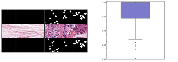
Fig. 3 (left) and 4 (right). In Fig. 3, the images in the upper row represent the pathologist-rendered masks; the middle row the original histopathological image; and the bottom row the images generated by the trained network. Each column represents all images associated with a single histopathological slide. The leftmost {3,3} grid portrays the three samples for which the trained network performed the best, in this all with 100% accuracy; the rightmost {3,3} grid portrays the three samples segmented with worst accuracy, in this case 92.2%, 93.4%, and 93.9% respectively. Fig. 10 portrays a box-and-whiskers plot; note the outliers.

Future Work

The results from the segmenting networks indicate that the relative frequency of the two classes categorized ("mask" or "not mask") impact the training and eventual performance of each network. In the case of the nuclei-segmenting network, this was particularly clear: while a very high (98.7% mean) pixelwise accuracy was achieved, a qualitative comparison of the testing set's masks and the final network's generated masks indicate that the network did not perform successful segmentation of individual nuclei as often as might be suspected. Indeed, the relative low frequency of the "mask" class (in other words, white pixels) suggests that the network was trained to favor the "non-mask" frequency in ambiguous cases.

This issue can be solved using so-called "mean frequency balancing", in which one generates class weights based on the relative number of pixels in the various classes. Specifically, mean frequency balancing coefficients are calculated by taking the ratio between the median of the class' frequency (computed on the entire training set) divided by the class' frequency.

Mean frequency balancing would also be a key step in solving the ultimate aim of the project: of creating a single network capable of segmenting multiple different types of cellular entities, as it would allow the network to segment various classes which vary widely in microscopy scale (or pixel frequencies).

Therefore, the next step is firstly to incorporate mean frequency balancing in the loss functions of the three above networks and re-train them on the datasets of their respective cell entities to see whether or not their segmenting accuracies improve. The second future task would be to create a single neural network with a mean frequency balanced loss function, train it on all the datasets, and see whether it can appropriately distinguish and segment tubules, epithelium cells, and nuclei.