Introduction

I set out with the goal of predicting regional electrical loads using neural networks. I didn't quite get there. However, I did create a set of tools to consume time series data into the Wolfram Language , transform the data into Time Series, Datasets and other structures necessary to analyze, visualize and predict Time Series data.

The Challenge

Predicting regional electrical loads and generation will become increasingly difficult as variable renewable resources such as solar photovoltaics and wind turbines account for a greater percentage of electrical generation. Regional electrical loads are influenced by a number of factors which render forecasting based on statistical techniques challenging. A visual inspection of summary data, and the load curves for a few individual days highlights some of the features that render traditional statistical tools challenging to work with.

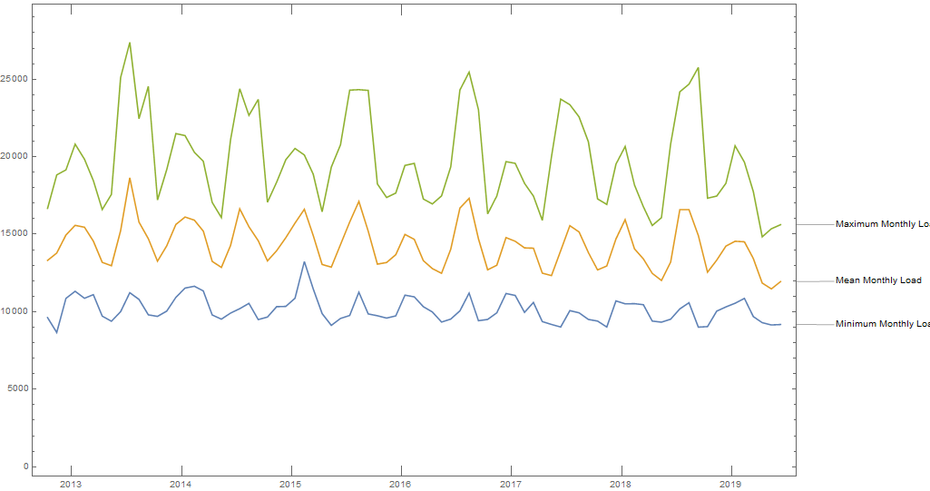The plot of minimum, mean and maximum load values by month illustrate that the time of year with the highest overall demand is the summer. Winter provides a second period of relatively high system load, while the system load during spring and autumn is relatively low.

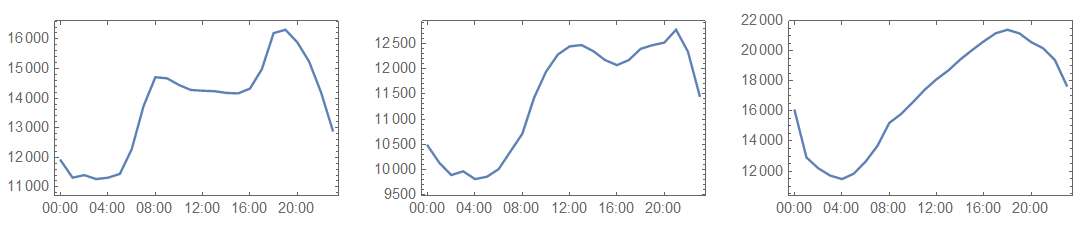The example load curves above illustrate that the daily load profile during the summer and winter months are quite different, and that the load curve during the milder months of the year share some features of summer and winter load curves.

These features, in addition to the impact of temperature, whether a day is a business day, the fact that the data is autocorrelated, and the fact that there are likely interactions between many of these terms makes determining the best statistical model to describe and forecast electrical load challenging. It was for these reasons that I was interested in using machine learning algorithms to predict regional electrical load.

Workflow

Acquiring and Importing System Load Data

Importing CSV files and Combining their Data

In the United States regional electrical operators, such as the New England Independent System Operator often make much of their load, generation and price data available for download from their website. I was able to download seven years of hourly system load data from the New England ISO's website as CSV files. An example file is attached to this post. The data was only available in 14 day increments, and each file had a number of header records and a trailer record. The function below will consume every CSV files in a directory named "data" within the notebook's directory, extract the data records from each file, and return a CSV file named "alldata.csv" that contains the complete data set.

https://www.iso-ne.com/isoexpress/web/reports/load-and-demand/-/tree/dmnd-rt-hourly-sys

importData[] := 
 importData @ 
  FileNames["*.csv", FileNameJoin[{NotebookDirectory[], "data"}]]
importData[csv_List] := Join @@ Map[importData, csv]
importData[path_String] := Module[
    {csv, headers, data},
    csv = Import[path, "CSV"];
    headers = csv[[6]];
    data = csv[[7 ;; -2]];
    Transpose[AssociationThread[headers -> Transpose[data]], 
    AllowedHeads -> All]
   ];
exportPath = FileNameJoin[{NotebookDirectory[], "alldata.csv"}];
data = importData[];
Export[exportPath, Join[{Keys[First[data]]}, Values[data]], "CSV"]

Combining Date and Hour Columns to a DateObject Comaptible Column

To create a TimeSeries in the Wolfram Language requires the time points in the series to be expressed in a format compatible with the DateObject function. This requires that the Date and HE (Hour Ending) columns in "alldata.csv" to be combined and reformatted. The functions below do this when applied to data in the "alldata.csv".

This function imports the "alldata.csv" as a Dataset object.

loadDataComplete=SemanticImport[ "C:\\filepath\\alldata.csv"]

This function transforms the "Date" and "HE" columns to DateObject and TimeObject,

loadDateObjectTimeObject = 
  loadDataComplete[All, {"Date" -> DateObject, "HE" -> TimeObject}];

This function creates a single column that combines the DateObject and TimeObject.

loadDataDateTime = 
  loadDateObjectTimeObject[
   All, (Append[#, "DateTime" -> DateObject[#Date, #HE]] &)];

Creating a TimeSeries

The TimeSeries within the Wolfram Language simplifies analysis, computation and visualization of time series data. It consists of a series of DateObject->Value pairs. The function below extracts each DateObject and Value pair from the Dataset defined by the prior function, and returns a TimeSeries object.

neISOLoad = TimeSeries @ Map[
    {#["DateTime"], #["MWh"]} &,
    Normal[loadDataDateTime]

You may find that there are gaps in your time series data. Many time series analyses are simplified if the data is regularly spaced. To create placeholders for each missing time point the TimeSeriesResample function can be used.

resampledNEISOLoad = TimeSeriesResample[neISOLoad, "Hour"]

Acquiring Weather Data

The Wolfram Language provides built in access to historical weather data. Since the system load data is for New England, I chose to download weather data for Boston, the largest city in the region. The weather data returned by the Wolfram Language is not regularly spaced, so the function below uses TimeSeriesRescale, and TimeSeriesResample to regularize the data into hourly intervals. Notice that the start and end times of the weather data time series are defined in terms of the "FirstDate" and "LastDate" of the system load data.

weatherData = TimeSeriesResample[
    TimeSeriesRescale[
      WeatherData["KBOS", 
    "Temperature", {resampledNEISOLoad["FirstDate"], 
     resampledNEISOLoad["LastDate"]}], 
      {resampledNEISOLoad["FirstDate"], resampledNEISOLoad["LastDate"]}
      ],
    "Hour"
    ]

Synthesizing Missing Weather Data and Load Data

The weather and load data have some missing values. The function below combines the two sets of data, and uses the built in SynthesizeMissingValues function to ensure that a value is available for each point in time in the TimeSeries.

loadandWeatherData = SynthesizeMissingValues@Transpose@{
     resampledNEISOLoad["Dates"], 
     resampledNEISOLoad["Values"], 
     Replace[weatherData["Values"], 
      Except[_Real | _Integer] :> Missing["Temperature"], {1}]
     };

Creating a BusinessDay and Hour column

The BusinessDayQ function applies a calendar definition to DateObject values, and returns True if the day is a Business Day and False if it is not. The default calendar is used here, but there are several built in Calendars, and one can define a custom calendar.

combinedWeatherLoadBusinessDay = Dataset @ Apply[
    <|
      "Date" -> #1, 
      "Temperature" -> #3,
      "Hour" -> TimeObject[#1],
      "BusinessDay" -> BusinessDayQ[#1],
      "Load" -> #2 
      |> &,
    loadandWeatherData,
    {1}
    ];

Transforming Data for Analysis

For the purpose of regression a number of the values in the data need to be transformed. The Date values need to be transformed to sequential integer values with 0 for the first value. The Hour column needs to be translated to an integer as well, and the BusinessDay column needs to be translated to 0 or 1. The following functions do this transformation, paired with the native Boole function are applied to the dataset below.

timeObjecttoHourInteger[hour_TimeObject] := DateValue[hour, "Hour"]
absoluteTimeDifferenceConverter[date_DateObject] := 
 QuantityMagnitude[
  DateDifference[resampledNEISOLoad["FirstDate"], date, "Hours"]]

datasetforregressionNOLAG = combinedWeatherLoadBusinessDay[All, {
   "Hour" -> timeObjecttoHourInteger,
   "BusinessDay" -> Boole,
   "Date" -> absoluteTimeDifferenceConverter}]

Introducing Lags to System Load Data

A common technique for the analysis of time series data is to introduce lagged values into the dataset. This allows statistical techniques to extract the relationship between a data point, and the points prior. Thirty lagged values were created, and the lagged values combined into a dataset.

To accomplish this the load values are extracted into a list, and a table is constructed where each row represents the System Load data lagged 1 time step. This creates lists that are longer than the original data set, by the number of lags introduced, so a function is applied to drop the first 30 time steps from the data. This expression extracts the System Load values into a list.

loadList = Normal[datasetforregressionNOLAG[All, "Load"]];

This expression creates a table of 30 lists of the System Load data, where the values in each subsequent list is shifted to the right.

shiftedLoadData = 
  Table[PadLeft[Drop[loadList, -i], Length[loadList]], {i, 30}];

The prior expression introduced 30 additional values in each list. To ensure that these lagged System Load Values have the same number of records as the actual System Load values, the following functions drop the first 30 values from each list.

drop30[list_List] := Drop[list, 30]
droppedShiftedLoadData = Map[drop30, shiftedLoadData];

This expression turns the table of lagged values created above, and returns a Dataset.

datasetofLaggedLoad = Dataset@Transpose[droppedShiftedLoadData];

This expression normalizes the Dataset that contains the load and temperature values.

normalData = Normal[datasetforregressionNOLAG];

This expression combines the lagged System Load values with the System Load, Temperature and Business day values.

mldata = Transpose @ Join[
        {
          normalData[[31 ;;, "Date"]], 
          normalData[[31 ;;, "Temperature"]], 
          normalData[[31 ;;, "BusinessDay"]]
        },
        droppedShiftedLoadData,
        {normalData[[31 ;;, "Load"]]}
    ];

The code shared in this post will allow you to consume time series data into the Wolfram Language from a CSV, and transform the data into TimeSeries, Datasets, and other structures. Once transformed the data can be analyzed using TimeSeriesModel and TimeSeriesForecast, Linear and Non-Linear regression or machine learning. My WSS 19 Final Project contains information on how to analyze the data using those methods.

Attachments:

alldata.csv

rt_hourlysysload...csv