Introduction
Tensors have wide applications in science and engineering. However, tedious index gymnastics often deter beginners and experienced researchers alike from grasping the physical meaning behind a string of tensors intuitively. The Penrose graphical notation was introduced by Roger Penrose to represent tensors by easily recognizable graphical objects that illustrate key structures at a glance. So far, no simple packages exist in the Wolfram language to convert tensor calculations to the Penrose graphical notations and vice versa. Thus, the aim of this project is to take tensor objects and their operations in the Wolfram language and visualize them using Penrose graphical notation. Here, we have created a package that parses a polynomial of tensor products and draws its graphical notation. A possible problem that might arise in the reverse direction may involve graph isomorphism problems because the Penrose graphical notation may not be unique and might require a sequence of transformations to turn a given diagram into default graphical standards. So it is not attempted in this project.
Crash Course on xAct
xAct is a Mathematica package for doing symbolic tensor calculations developed by José M. Martín[Minus]García. First, let us load the package
<< xAct`xTensor`
To make a tensor, we have to first define the manifold on which it resides :
DefManifold[M3, 3, {a, b, c, d, e, f, g}]
** DefManifold: Defining manifold M3.
** DefVBundle: Defining vbundle TangentM3.
This is a three dimensional manifold with seven slots for indices, which tensors residing on it can use. To define the tensor T with some covariant and contravariant indices living on M3,
DefTensor[T[-a, b, -c, d, -e, f, -g], M3]
** DefTensor: Defining tensor T[-a,b,-c,d,-e,f,-g].
However, every instance of the tensor of this form can have any number and pattern of indices, as long as it follows the constraints given by the above definition. For example,
T[-a, b, -c, c]
will return $T^{\ b\ c}_{a\ c}$. This is a valid construction under the above definition. This is a tensor with two covariant (lower) indices "a" and "c", and two contravariant (upper) indices "b" and "c", with no symmetry specified.
The Penrose Graphical Notation
The Penrose graphical notation is a set of symbols, that when combined, can be used to describe almost all tensorial equations and statements visually. For instance, on Wikipedia, one may find that 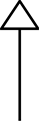 a contravariant vector
 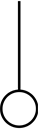 a covariant vector
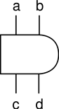 a rank 4 tensor with two contravariant and two covariant tensors
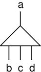 a rank 4 tensor with one contravariant and three covariant tensors.
Design Principles
To visualize tensors, we need to make graph objects. To make everything simple, we opt not to use customized shapes for the head of the tensors, but use a standard boxed frame:
tensorShape[s_][x_, _, _] :=
 Inset[Framed[
   Style[s, TextAlignment -> Center, Medium, FontFamily -> "Times",
    Italic, Black], Background -> LightBlue, RoundingRadius -> 5], x]
, where "s" is the tensor head to be displayed, for instance, $T^{\ b\ c}_{a\ c}$. The tensorShape function takes a curried form, where the arguments are separated into two groups--the first argument is for the text we put in, and the second list of arguments including the empty slots are reserved for the VertexShapeFunction to fill in when constructing the graph.
The input expression we consider is a tensorial polynomial, which means a linear combination of tensor products. We will construct a function that makes a graph object for each atomic/non-tensor-product type tensor called makeGraph, and a function that adds the tensor product notation $\otimes$ to each position where a tensor product takes place, called addTensorProduct. Then the final function tensorVisualize substitutes the graphs for atomic tensors in the original polynomial and display the expression as a graphics object of polynomial of tensors.
makeGraph
makeGraph[tensor_, outputContract_:False]:=Module[
{upIdx,downIdx,upEdgeList,downEdgeList, edgeList,vertexList,legList,upLabelList,downLabelList,graph,contractVertex},
upIdx = IndicesOf[Up][Evaluate@tensor]/.IndexList->List;
downIdx = IndicesOf[Down][Evaluate@tensor]/.IndexList->List;
downEdgeList = Normal@AssociationMap[0&,downIdx];
upEdgeList = Reverse[#,2]&@Normal@AssociationMap[0&,upIdx];
edgeList = Join[downEdgeList,upEdgeList];
legList=FindIndices@Evaluate@tensor;
vertexList =Append[legList,0];
upLabelList=Normal@AssociationThread[DirectedEdge@@@upEdgeList,Placed[#,"End"]&/@(Style[#, Medium, FontFamily -> "Times", Italic, Black]& )/@ToString/@upEdgeList[[All,2]]];
downLabelList=Normal@AssociationThread[DirectedEdge@@@downEdgeList,Placed[#,"Start"]&/@(Style[#, Medium, FontFamily -> "Times", Italic, Black]& )/@ToString/@-downEdgeList[[All,1]]];
graph=Graph[DirectedEdge@@@edgeList,GraphLayout->{"RadialEmbedding","RootVertex"->0},VertexShapeFunction->{0->tensorShape[tensor//StandardForm],None},VertexSize->0.45,
VertexLabels->None,PerformanceGoal->"Quality",EdgeLabels->Join[upLabelList,downLabelList]];
If [
IntersectingQ[upIdx,-downIdx],
contractVertex=Intersection[upIdx,-downIdx];
graph =VertexContract[graph,#]&@Thread[{contractVertex,-contractVertex}];
If[
outputContract,
contractVertex,
EdgeAdd[graph,DirectedEdge[0,0],EdgeLabels->Join[Options[graph,EdgeLabels][[1,2]],{DirectedEdge[0,0]->StringRiffle[contractVertex,", "]}]]
]
,graph
]
]
The IndicesOf and FindIndices are functions from xAct that returns the list of indices of the tensor, with which we build a list of edges that will constitute the graph. For the head of the tensor, we by convention set its vertex to be "1". Then we distinguish contra- and covariant indices by using DirectedEdge. All edges that go from the vertex representing the index to "1" are covariant, and all edges that go from "1" to the indices are contravariant. So for example, if we have a tensor with a contravariant index "a", and two covariant indices "b" and "c", then the list of edges are
DirectedEdge @@@ {{1, a}, {b, 1}, {c, 1}}
{1 \[DirectedEdge] a, b \[DirectedEdge] 1, c \[DirectedEdge] 1}
For tensors that have repeating indices that appear both in the top and the bottom, the indices will be contracted according to the Einstein summation rule. So if the original tensor has rank n, the contracted tensor will have rank n-2. To take contraction into account, we used VertexContract to remove the edges that represent indices to be contracted. Then we add a self-directed loop to goes from "1" to "1" to represent all the contracted indices.
addTensorProduct
addTensorProduct[tensor_]:=Replace[tensor,(HoldPattern[Times[pre___,tensors:Repeated[_?(xTensorQ[Head[#]]&),{2,Infinity}]]]):>Times[pre,CircleTimes[tensors]],Infinity]
, where xTensorQ is a function from xAct that tests whether the head of an expression is a tensor that has been defined. This function searches for occasions where two or more tensor objects are multiplied together and inserts a tensor product symbol $\otimes$ in between.
replaceByGraph
replaceByGraph[tensor_]:=tensor/.t_?(xTensorQ[#[[0]]]&):> Show[makeGraph@t,ImageSize->Medium]
This function replaces all the atomic tensor expressions by their graphical representation produced by makeGraph. It looks for all expression that has a tensorial head using
_?(xTensorQ[#[[0]]] &)
and maps the tensor to the graph using RuleDelayed.
tensorVisualize
tensorVisualize[tensor_,size_:60,simple_:True]/;BooleanQ[simple]:=If[
simple,
Style[#,FontSize->size]&@replaceByGraph@addTensorProduct@Simplification@tensor,
Style[#,FontSize->size]&@replaceByGraph@addTensorProduct@tensor
]
This function composes the functions above and visualizes a polynomial of tensor products, with the option to view the simplified version returned xAct.
Examples
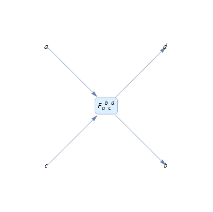
tensorExpr = T[-a, b, -c, d]
tensorVisualize@tensorExpr
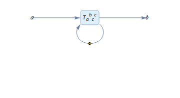
tensorExpr1 = T[-a, b, -c, c]
tensorVisualize@tensorExpr1
Let us build a polynomial of tensors and see how it can be visualized. First, we can define some other tensors, say DefTensor[G[a, -b, -c, d, -e, f], M3] ** DefTensor: Defining tensor G[a,-b,-c,d,-e,f].
DefTensor[v[a], M3]
** DefTensor: Defining tensor v[a].
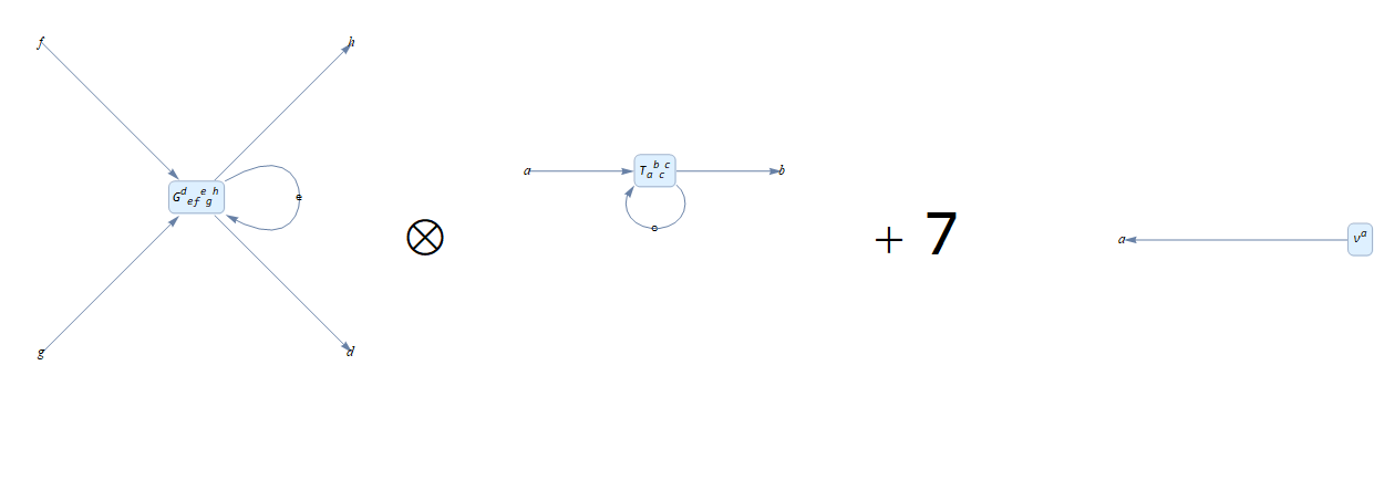
tensorExpr2 = T[-a, b, -c, c] G[d, -e, -f, e, -g, h] + 7*v[a]
If we visualize this tensor with the default option, where simplification from xAct is turned on, then it will return:
tensorVisualize[tensorExpr2]
Validate::inhom: Found inhomogeneous indices: {IndexList[a], IndexList[-a, b, d, -f, -g, h]}.
Throw::nocatch: Uncaught Throw[Null] returned to top level.
, because the tensor polynomial is not a validate expression. A valid tensor polynomial must be homogenous, that is, all tensor products being summed up must have the same rank. This is not the case here, nonetheless, we can visualize this ill-defined tensor by turning off the simplification option:
tensorVisualize[tensorExpr2, 60, False]
Future Work
A tensor can always be written as the sum of a symmetric part and an antisymmetric part. Therefore, it is crucial to also include a feature that indicates whether the tensor is symmetric or antisymmetric under a transposition of any given pair of indices of the tensor. This feature is so far half-complete and will be updated on the community post once finished.
My GitHub Link
 Attachments:


