Goal of the project

The goal of the project was to improve importance sampling in Monte Carlo integration of sharp functions using invertible neural network as a sampler. Invertible neural networks are state of the art when it comes to generating new samples of data.

Background

In Monte Carlo integration we estimate a definite integral of a function $f(x)$ by randomly choosing points over which the integral is evaluated.

Importance sampling aims to estimate an expected value of a function $f(x)$ , while only having samples generated from a different distribution than the distribution of interest. The intuiton behind it is that we want to place higher density of points in region where integrand is large.

$$ \mu_q = \frac{1}{n}\sum_{i=1}^n f(\textbf{x}_i) \frac{p(\textbf{x}_i)}{q(\textbf{x}_i)} $$

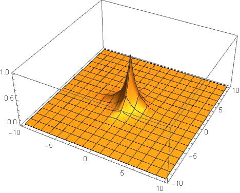
We picked a simple function to test our model on with a domain to integrate over

functionToIntegrate = Function[Exp[-(Abs[#1]+Abs[#2])]];
domain = {{-10,10},{-10,10}};

Importance sampling is particularly useful for sharp functions which are mostly zero except a single sharp region. This sharp region contributes the most to the integrand so we are interested in sampling from it rather than sampling from areas where function is zero.

Functions for Monte Carlo integration with importance sampling

To enable running multiple experiments we wrote a function to sample with a neural network. It evaluates the function at all samples and assigns weights to them. These weights are then used for resampling from the distribution learned with an invertible neural network.

ImproveSampling[{x_, xPDF_}, {f_, domain_}, numSamples_] := Module[
    {ld,values, learnedSamples, z, zPDF, importanceWeights, pos, resampled},
    (* Resample with more weight given to the samples from higher values of f*)
    importanceWeights = Abs[f @@@ x] / xPDF;
    resampled = RandomChoice[importanceWeights -> x, numSamples];
    ld = LearnDistribution[resampled, Method -> "RealNVP", PerformanceGoal->"DirectTraining"];
    (* Sample from the learned distribution and mix it with uniform distribution for non-unitary weights*)
    z = If[weight === 1,
       RandomVariate[ld, numSamplesMonteCarlo],
       Join[RandomVariate[ld,Ceiling[numSamples * weight]],RandomVariate[UniformDistribution[domain], Floor[numSamples * (1-weight)]] ]
    ];
    (* Delete the points sampled with the neural network that are not in the domain of integration*)
    pos = Position[z, pt_ /; Not[domain[[1,1]]< First[pt] <domain[[1,2]] && domain[[2,1]]< Last[pt] <domain[[2,2]]], {1}, Heads -> False];
    z = Delete[z, pos];
    (* Find the probability distribution function (PDF) for the improved samples *)
    zPDF = If[weight === 1,
       PDF[ld, z],
       Quiet[PDF[ld, z] * weight + PDF[UniformDistribution[domain], z] * (1-weight), General::munfl]
    ];

    {z,zPDF}
];

In our experiment the neural invertible network we used was RealNVP. RealNVP Real NVP implements a normalizing flow for density estimation.

With each sampling iteration we should track the error off the importance sampling, i.e. the deviation from the Monte Carlo estimated integral and the true value of the integral. We may find it using the equation above.

Evaluation[{x_, xPDF_}, {f_, domain_}] := Module[
    {p, values, domainSize, MCIntegral, trueIntegral},
    (* 1. Compute the integral with Monte Carlo *)
    p = PDF[UniformDistribution[domain], x];
    values = f @@@ x;
    domainSize = (Abs[domain[[1,2]] - domain[[1,1]]]) * (Abs[domain[[2,2]] - domain[[2,1]]]);
    MCIntegral = Mean[values * p / xPDF] * domainSize;
    (* 2. Estimate the deviation to the real value *)
    trueIntegral = NIntegrate[f[x1, x2],  Flatten @ {x1, domain[[1]]}, Flatten @ {x2, domain[[2]]}];
    Abs[MCIntegral - trueIntegral]
]

Results

We run several experiments sampling from a uniform distribution at the first iteration and passing the output of each improved sampling to the next iteration thereof.

mainExperiment[functionToIntegrate_, domain_, weight_, numSamplesMonteCarlo_,numSamplesLearnDistribution_, iter_:5] := Module[
    {samples, pdfSample,results, sampleList},
    SeedRandom[196]; (* for reproducibility *)

    samples =  RandomVariate[UniformDistribution[domain], numSamplesMonteCarlo];
    pdfSample= PDF[UniformDistribution[domain], samples];
    results = {Evaluation[{samples, pdfSample}, {functionToIntegrate, domain}]};
    sampleList = {samples};

    Do[
    (* Improve *)
    {samples, pdfSample} = ImproveSampling[{samples, pdfSample}, {functionToIntegrate, domain}, numSamplesLearnDistribution];

       If[Length[samples] == 0,
         Echo["No sample in the domain!"];
         Break[]
       ];

       (* Evaluate *)
       AppendTo[results, Evaluation[{samples, pdfSample}, {functionToIntegrate, domain}]];
       AppendTo[sampleList, samples];
       , iter
       ];
    <| "absoluteError" -> results, "samples" -> sampleList |>

];

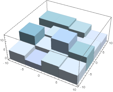
After several iterations of improved sampling with neural networks the samples are mostly from the sharp region which contributes the most to the integrand.

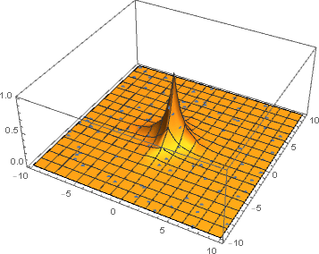
By plotting a histogram, we can clearly see that the spike of the function is learned very quickly. At next iterations the invertible neural network learns to sample more from the region where the function is sharp and less from the region where it is close to zero.

By sampling only 100 points each time, we already observed good error convergence at five iterations of improved sampling.

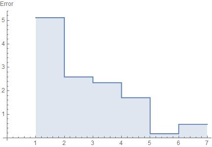
We also explored the correspondence between the size of the domain and the number of samples required for good Monte Carlo estimation of the integral. Let us plot how the error changes with number of samples varied from 20 to 500 and the size of domain varied from 500 to 10000. A small domain chosen just around the peak of the function and a large number of samples should give the smallest error.

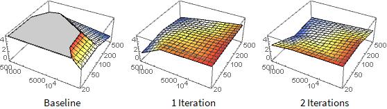
As expected the largest error (red) corresponds to a small number of samples and a large domain size.

Future work

The future work could involve integrating different sharp functions and using different mixtures of distributions during sampling. We used a mixture of uniform and the one sampled with a neural network but we have yet to explore mixture of Gaussians. We could also use our model for Monte Carlo integration for functions of arbitrary dimensions.

Another obvious development yet to be made is finishing the Invertible Residual Network implementation which we initially planned to do. This is the latest state of the art model in generative modeling and density estimation.