Introduction

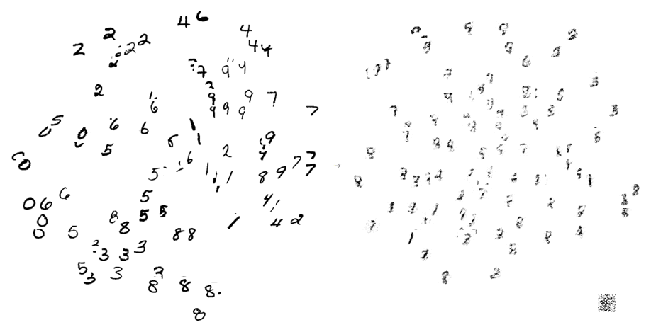
Given a set of images, we train a neural network to learn the distribution from which these images are represented then use this distribution to generate images that look like those in the dataset. We then use transfer learning to see how well the network can generate images it has not seen before given only a few examples.

For this project we will use the MNIST dataset. We first try to learn the latent space of the data which consists of the digits 0 to 8, then invert elements from the latent space back to the data space to generate new data. We will then show our neural network few examples of the digit 9, which it has never seen before, and see how well it performs the task of generating new 9's. Surprisingly, the results were better than expected.

Some Theory

Given an observed data variable $x \in X$, a simple prior probability distribution $p_{Z}$ on a latent variable $z \in Z$, and a bijection $f : X \rightarrow Z$ with $g=f^{-1}$, the change of variable formula defines a model distribution on $X$ by

$$\begin{align} p_{X}(x) &= p_{Z}(f(x))\left|\operatorname{det}\left(\frac{\partial f(x)}{\partial x^{T}}\right)\right| \\ \log \left(p_{X}(x)\right) &= \log \left(p_{Z}(f(x))\right)+\log \left(\left|\operatorname{det}\left(\frac{\partial f(x)}{\partial x^{T}}\right)\right|\right) \end{align} $$

where $\frac{\partial f(x)}{\partial x^{T}}$ is the Jacobian of $f$ at $x$. The function $f$ here is the neural network.

A sample $z \sim p_{Z}$ is drawn in the latent space, and its inverse image $x=f^{-1}(z)=g(z)$ generates a sample in the original data space.

The MNIST data

We will use the MNIST dataset which consists of 60000 examples of grayscale images of handwritten digits ( $28\times28$ pixels). We first import the data then take only examples with the digits 0 to 8.

digits08 = Cases[ResourceData["MNIST"], Except[_ -> 9]][[All, 1]];

Training

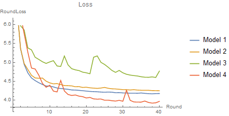
For training on the dataset, we use LearnDistribution[] which will attempt to understand the underlying distribution for the given data. The method used will be RealNVP for which we will attempt four different hyper-parameter configurations. We will then select the best model to perform our transfer learning task. The best performing model that we used, given computational resources and time was the following:

ldtrial4 = LearnDistribution[digits08, 
  Method -> {"RealNVP", "NetworkDepth" -> 4, 
    "CouplingLayersNumber" -> 4, MaxTrainingRounds -> 100, 
    "ActivationFunction" -> Ramp}, 
  PerformanceGoal -> "DirectTraining"];

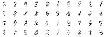
From this model, we can easily take generated samples of the digits.

Grid[{RandomVariate[ldtrial4, 10], RandomVariate[ldtrial4, 10], 
  RandomVariate[ldtrial4, 10], RandomVariate[ldtrial4, 10]}]

Here we can already see that the network is able to decently generate images that look like digits from MNIST. These results are great considering the fact that we used 30 minutes of training time on one GPU. We can compare the performance of this model where we used a network depth = 4, coupling = 4, and ReLU activation (Model 4).

Transfer Learning

We would like to use features already learned in our model to generate a good representation of the digit 9. Note that our model has not yet seen the digit 9. We will now show our model only ten examples of the digit 9 then try to generate these 9's by mapping from the latent space → data space.

New data and model

First, we import data from MNIST with the digit 9 only.

digit9 = Cases[ResourceData["MNIST"], HoldPattern[_ -> 9]] [[All, 1]];

Next, we take only 10 examples for which we will use to train.

sampledigit9 = RandomSample[digit9, 10]

As a baseline comparison, let's look at what happens if we just train the model without transfer learning.

ld9 = LearnDistribution[sampledigit9, 
   Method -> {"Multinormal", "IntrinsicDimension" -> 10, 
     "CovarianceType" -> "Diagonal"}, PerformanceGoal -> "Quality"];

The model generated images that look like the digit 9.

However, we can do better with transfer learning. First, we will learn the latent space of the digit 9 then input elements from this space to generate the data space using our RealNVP model.

Mapping to Latent space $X\to Z$

The following block of code will convert our data $x$ to elements in the latent space $z$.

checkeredGen[inpdim_, checkeredType_, mreplicat_] := Module[
    {resLayer, replayer, checkerf},
    replayer = ReplicateLayer[mreplicat];
    checkerf = If[Depth@inpdim > 1,
       resLayer = ReshapeLayer[inpdim];
       {Normal@SparseArray[{{i_, j_}/; Switch[checkeredType, "black", OddQ[i + j], "white", EvenQ[i + j]] == True -> 1}, inpdim]},
       resLayer = ReshapeLayer[{inpdim}];
       {Normal@SparseArray[{{i_}/; Switch[checkeredType, "black", OddQ[i], "white", EvenQ[i]] == True -> 1}, inpdim]}
       ];
    checkerf = resLayer@checkerf;
    Normal[replayer[checkerf]]
]
pp = ldtrial4[[1, "Preprocessor"]];
p = ldtrial4[[1, "Processor"]];
mpr = ldtrial4[[1, "Model", "Processor"]];
mppr = ldtrial4[[1, "Model", "PostProcessor"]];

trainednet allows us to input samples from the data space and generate the latent space of our model: trainednet = ldtrial4[[1, "Model", "ProbabilityNet"]]

sampler will allow us to input elements of the latent space and generate MNIST digits.

sampler = ldtrial4[[1, "Model", "Sampler"]]

nn = trainednet[["Input"]];
mm = Length@sampledigit9

nn and mm will give the dimensions of our data. Since we only use ten examples of the digit 9, and each example are $28\times28$ pixels, the dimensions will be $(10\times784)$.

{mm, nn} = Dimensions@mppr[p[pp[sampledigit9]]]
{10, 784}

checkerW = checkeredGen[nn, "white", mm];
checkerB = checkeredGen[nn, "black", mm];

Dimensions@checkerW
{10, 784}

Finally, we define z9 to be our latent variable:

z9 = trainednet[<|"Input" -> mppr[mpr[p[pp[sampledigit9]]]], 
     "checker_w" -> checkerW, "checker_b" -> checkerB|>][["Z_out"]];

Training

We now learn the distribution of the latent space, then take samples from this space and input them into our RealNVP model to see how well we can generate the digit 9.

ld9 = LearnDistribution[z9, 
   Method -> {"Multinormal", "IntrinsicDimension" -> 10, 
     "CovarianceType" -> "Diagonal"}, PerformanceGoal -> "Quality"];

sampledz = RandomVariate[ld9, 10];

Mapping to data space $Z\to X$

Finally, we use the latent space to generate the digit 9.

gen9=pp[p[mpr[mppr[
sampler[<|"Input" -> sampledz, "checker_w" -> checkerW, 
"checker_b" -> checkerB|>], "Inverse"], "Inverse"], 
"Inverse"], "Inverse"]

As you can see, the results are much better than before!

Transformations

The following animation shows the transformation between data and latent spaces. We transform the digit 2 to an 8.

$2\to Z \to 8 \to Z \to 2$

Further Work

In the future, we plan to

• Perform better hyper-parameter tuning on the network to improve performance.
• Add convolutional layers to the Real NVP network which is expected to improve generation accuracy tremendously.
• Fully implement an invertible residual network which will provide a much more accurate representation of the latent space and generate the data space more efficiently.

Acknowledgements

Many thanks to Etienne Bernard, Jerome Louradour, and Amir Azadi for their help and support in successfully completing this project.