Real Physical Networks of Time-Dependent Neurons:
Differential Equation Neuron Networks or: DiffyQNet

Fig 1: XOR in-training (synapse-based)
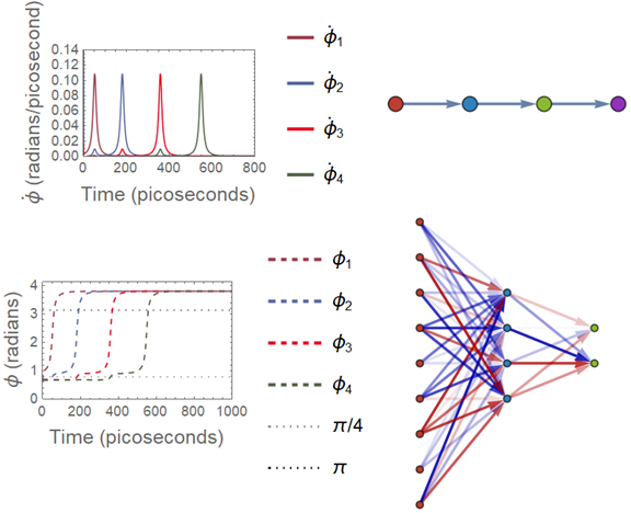
Fig 2: Plots of Rate & State; Plotted Architecture & Fully Connected Net Example
Preamble
For posterity, and to help future Wolfram Summer School attendees, there are two introductions/abstracts available at the end of this post: (Before WSS19) is prior to my entrance into WSS19, and (After WSS19) is after the project reached a point of metastability at the finish of the WSS19 program.
Introduction
In this project, coupled sets of time-dependent 2nd order ordinary differential equations (DiffyQs) describing the spiking behavior of certain orientations of materials forming a physical neuron network are simulated based on their given material parameters. These DiffyQNets are trained through an iterative stochastic-gradient-descent-like method wherein the algorithm proceeds as such:
(1) Chosen random output index from a randomly selected input vector is simulated.
(2) Error is computed by comparison of simulated output against desired outcome.
(3) Update to current vector/connectivity array made by combination of specified learning rate with the error computed in (2) to aid in convergence.
(4) Method is ceased after a defined number of iterations.
This implemented functionality consists of a set of functions: DiffyQNet, DiffyQNetSim, DiffyQNetTrainSynapse, DiffyQNetTrainCurrent, DiffyQNetPlotRate, and DiffyQNetPlotState.
In the investigated case, DiffyQNet dictates the behavior of a bilayer of an antiferromagnet (AFM) and a normal metal (NM) using a DiffyQ described in [1-2]. Then, DiffyQNetSim simulates the results of application of DiffyQNetTrainSynapse on the system. Finally, the resulting actions of the system are shown using DiffyQNetPlotRate and DiffyQNetPlotState.
Starting Point & Initial Issues
The functions of these artificial neurons are time-based and cannot be used within the existing Neural Network framework. As such, it became necessary structures mimicking the functionality of the existing framework, namely: NetChain, NetGraph, NetTrain, etc.
DifferentialEquationNetworks
DifferentialEquationNet
This function is the basis of the project, here, we construct a 2nd order ordinary differential equation in order to describe the behavior of our neurons we will build into a network. It can be called by doing the following:
SynapseMatrix = .01*Normal[SparseArray[Band[{2, 1}] -> 1, {4, 4}]];
Current = ConstantArray[.974, 4];
DiffyQNet[SynapticMatrix,Currents]
The results are set into an association, for ease of calling the needed values with keys. Explanation of inputted terms will be included at a later date, or upon request if desired sooner.
<|"Equations" -> {0.00549779 Sin[2 Subscript[?, 1][t]] +
 0.1 Derivative[1][Subscript[?, 1]][t] +
 0.00578745 (Subscript[?, 1]^??)[t] ==
0.00535484,
0.00549779 Sin[2 Subscript[?, 2][t]] +
 0.1 Derivative[1][Subscript[?, 2]][t] +
 0.00578745 (Subscript[?, 2]^??)[t] ==
0.00535484 + 0.01 Derivative[1][Subscript[?, 1]][t],
0.00549779 Sin[2 Subscript[?, 3][t]] +
 0.1 Derivative[1][Subscript[?, 3]][t] +
 0.00578745 (Subscript[?, 3]^??)[t] ==
0.00535484 + 0.01 Derivative[1][Subscript[?, 2]][t],
0.00549779 Sin[2 Subscript[?, 4][t]] +
 0.1 Derivative[1][Subscript[?, 4]][t] +
 0.00578745 (Subscript[?, 4]^??)[t] ==
0.00535484 + 0.01 Derivative[1][Subscript[?, 3]][t]},
"InitialConditions" -> {{0.671132, 0.671132, 0.671132, 0.671132}, {0,
 0, 0, 0}}, "ClockPeriod" -> 2500,
"AnisotropicFrequecy" -> 0.0109956, "EffectiveDamping" -> 0.1,
"ExchangeFrequency" -> 172.788, "NumberNeurons" -> 4,
"ConnectivityMatrix" -> {{0., 0., 0., 0.}, {0.01, 0., 0., 0.}, {0.,
0.01, 0., 0.}, {0., 0., 0.01, 0.}},
"NetworkCurrent" -> {0.974, 0.974, 0.974, 0.974}|>
This will be apparent later on, in the way further functions are called and interact with one another.
DifferentialEquationNetSim
This function will simulate the behavior of the constructed DiffyQNet. From here, we can test the behavior of the network before and after training with DiffyQNetTrain.
DiffyQNeuralNetwork = DiffyQNet[SynapseMatrix, Current];
BinaryInput={{1}};
DiffyQNetSim[DiffyQNeuralNetwork, {{1}}]
The results, again in an association, allow for the examination of the outputted behavior of the system.
<|"EndConditions" -> {{{3.81272, 3.81272, 3.81272,
     3.81272}, {-7.56906*10^-19, -1.86168*10^-18, 1.14884*10^-17,
     1.58353*10^-15}}}, "BinaryOutput" -> {{1, 1, 1, 1}},
 "DeltaStrength" -> {0.01, 0, 0, 0}|>
This can all seem a bit confusing, at first, but with time, the obvious behaviors of such a simple system will become apparent. If not, the use of DiffyQNetPlotState and DiffyQNetPlotRate can readily provide a visual explanation of the occuring behaviors:
StartingConditions =
  Join[{DiffyQNeuralNetwork["InitialConditions"][[1]],
    DiffyQNeuralNetwork["ExchangeFrequency"]*Pi*{.01, 0, 0, 0}}];
rate = DiffyQNetPlotRate[DiffyQNeuralNetwork, StartingConditions,
  800, .14, 0]
state = DiffyQNetPlotState[DiffyQNeuralNetwork, StartingConditions,
   1000, Pi + 1, 0]["StatePlot"]
As can be seen in the DiffyQNetPlotState associations can again be used to access the state plot, versus a collection of the adjusted weights during training, as was used in the creation of the GIF at the top of this post. The outputs from the following are seen on the left side of Fig. 2, with the rates showing the spiking behavior of the neurons, and the states showing the corresponding angle of the Néel vector as discussed in the reference papers.
DiffyQNetTrain(Synapse & Current)
While the above example is a simple one, seen in the upper right of Fig. 2, more complex systems such as AND, OR, XOR, and Fully Connected Networks (FCN) can be made. For the use of FCN for classification purposes, encoders must reach a finalized stage of construction, and their uses will be described in subsequent publications regarding MNIST classification. Here, however, it can be shown that AND, OR, and XOR gates are easily constructed and trained. An example of AND & OR, while sharing identical initial geometries, appropriately show the wide versatility of this DiffyQNet system.
ANDmat = ORmat = {{0, 0, 0, 0, 0}, {0, 0, 0, 0, 0}, {.01, 0, 0, 0,
     0}, {0, .01, 0, 0, 0}, {0, 0, .01, .01, 0}};
TrainedAND =
  DiffyQNetTrain[
   DiffyQNet[ANDmat,
    ConstantArray[.974, 5]], {{1, 0}, {0, 1}, {1,
     1}}, {{0}, {0}, {1}}, 30];
(DiffyQNetSim[TrainedAND["TrainedNet"], {{1, 0}, {0, 1}, {1, 1}}][
   "BinaryOutput"])[[1 ;;, {1, 2, 5}]]
{{1, 0, 0}, {0, 1, 0}, {1, 1, 1}}
TrainedOR =
  DiffyQNetTrain[
   DiffyQNet[ORmat,
    ConstantArray[.974, 5]], {{1, 0}, {0, 1}, {1,
     1}}, {{1}, {1}, {1}}, 30];
(DiffyQNetSim[TrainedOR["TrainedNet"], {{1, 0}, {0, 1}, {1, 1}}][
   "BinaryOutput"])[[1 ;;, {1, 2, 5}]]
{{1, 0, 1}, {0, 1, 1}, {1, 1, 1}}
The differences in the structures can be seen with the appropriate key usage.
TrainedOR["TrainedNet"]["ConnectivityMatrix"]
{{0, 0, 0, 0, 0}, {0, 0, 0, 0, 0}, {0.01, 0, 0, 0, 0}, {0, 0.01, 0, 0, 0}, {0, 0, 0.01, 0.01, 0}}
TrainedAND["TrainedNet"]["ConnectivityMatrix"]
{{0, 0, 0, 0, 0}, {0, 0, 0, 0, 0}, {0.01, 0, 0, 0, 0}, {0, 0.01, 0, 0, 0}, {0, 0, 0.005, 0.005, 0}}
Current Training can also occur with similar syntax, but this time, the connectivity matrices are held static, and the current level of the neurons is what is adjusted.
currentTrainedAND =
  DiffyQNetTrainCurrent[
   DiffyQNet[ANDmat,
    ConstantArray[.974, 5]], {{1, 0}, {0, 1}, {1,
     1}}, {{0}, {0}, {1}}, 30];
(DiffyQNetSim[
    currentTrainedAND["TrainedNet"], {{1, 0}, {0, 1}, {1, 1}}][
   "BinaryOutput"])[[1 ;;, {1, 2, 5}]]
{{1, 0, 0}, {0, 1, 0}, {1, 1, 1}}
currentTrainedOR =
  DiffyQNetTrainCurrent[
   DiffyQNet[ORmat,
    ConstantArray[.974, 5]], {{1, 0}, {0, 1}, {1,
     1}}, {{1}, {1}, {1}}, 30];
(DiffyQNetSim[
    currentTrainedOR["TrainedNet"], {{1, 0}, {0, 1}, {1, 1}}][
   "BinaryOutput"])[[1 ;;, {1, 2, 5}]]
{{1, 0, 1}, {0, 1, 1}, {1, 1, 1}}
Helper Functions
Many of the visualizations of the Architecture and Weights can be made with the following helper functions:
GraphLayerList
GraphLayerList[inpmat_] :=
 Module[{glist =
    Join @@ MapIndexed[
      Thread@DirectedEdge[
         First /@ Position[#1, Except[0 | 0.], {1}, Heads -> False],
         First@#2] &, inpmat], classes = {}, classvrtcs},
  classvrtcs =
   Cases[Thread[{VertexList@glist, VertexInDegree@glist}], {v_, 0} :>
     v];
  While[Length@classvrtcs > 0
   ,
   AppendTo[classes, Union@classvrtcs];
   classvrtcs =
    Cases[EdgeList@
      glist, (Alternatives @@ Last[classes]) \[DirectedEdge] v_ :> v]
   ];
  {glist, classes}
  ]
ColPacity Style
ColPacity[adjmat_, poscol_, negcol_] := Block[{styleEdge},
   (
    styleEdge[n_Real] := {Opacity[50 Abs@n],
      If[Positive[n], poscol, negcol], Thick};
    Map[# -> styleEdge@Part[adjmat, #[[2]], #[[1]]] &,
     GraphLayerList[adjmat][[1]]]
    )];
ADJmatFCN
ADJmatFCN[numinput_, numoutput_, numtotal_, defaultweight_: .01] :=
 Module[{numhidden = numtotal - numinput - numoutput},
  defaultweight*
   Normal@SparseArray[{Band[{numinput + 1, 1}, {numinput + numhidden,
         numinput}, {1, 1}] -> {{1, 1}, {1, 1}},
      If[numhidden != 0,
       Band[{numinput + numhidden + 1, numinput + 1}, {numtotal,
          numinput + numhidden}, {1, 1}] -> {{1, 1}, {1, 1}},
       Nothing]}, {numtotal, numtotal}]]
StyledGraphPlotter
Options[StyledADJPlot] = {"PositiveColor" -> Darker@Red,
   "NegativeColor" -> Darker@Blue};
StyledADJPlot[adjmat_, OptionsPattern[]] :=
 Block[{amat = adjmat, poscol = OptionValue["PositiveColor"],
   negcol = OptionValue["NegativeColor"]},
  LayeredGraphPlot[GraphLayerList[adjmat][[1]], Left,
   VertexStyle ->
    Flatten@MapIndexed[#1 -> ColorData[63][#2[[1]]] &,
      GraphLayerList[adjmat][[2]], {2}], VertexSize -> 0.2,
   EdgeStyle -> ColPacity[amat, poscol, negcol],
   AspectRatio -> GoldenRatio]]
Results & Future Work
We find that AND, OR, and XOR gates can be efficiently simulated using the NDSolve framework, with over 200 iterative computations of networks consisting of several coupled neurons having little impact on the required computation time, occurring in under 3 seconds. This shows that the application & training of similar networks to the classification of larger systems like the MNIST database which are still comparatively smaller in size to other datasets will not be temporally expensive to perform. These expedient results thus provide impetus to the continued development of this project for generalized time-dependent DiffyQNets.
Future Development Plans
Functions will continue to be built out into a complete system, and inevitably released in packaged form through github, and available individually from the Wolfram Language Function Repository. Links will be provided in this section and elsewhere once these are made available. (07/10/19 not currently available)
Before/After Abstracts
(After WSS19)
Title:
Differential Equation Neural Networks:
(DiffyQNet) From artificial digital time-independent neurons to real physical time-dependent neurons
(A necessary first step towards innovative computing paradigms)
Author(s):
CA Trevillian
Project Description:
In this project, coupled sets of time-dependent 2nd order ordinary differential equations (DiffyQs) describing the spiking behavior of certain orientations of materials forming a physical neuron network are simulated based on their given material parameters. These DiffyQNets are trained through an iterative stochastic-gradient-descent-like method wherein the algorithm proceeds as such:
(1) Chosen random output index from a randomly selected input vector is simulated.
(2) Error is computed by comparison of simulated output against desired outcome.
(3) Update to current vector/connectivity array made by combination of specified learning rate with the error computed in (2) to aid in convergence.
(4) Method is ceased after a defined number of iterations.
This implemented functionality consists of a set of functions: DiffyQNet, DiffyQNetSim, DiffyQNetTrain, DiffyQNetPlotRate, and DiffyQNetPlotState. In the investigated case, DiffyQNet dictates the behavior of a bilayer of an antiferromagnet (AFM) and a normal metal (NM) using a DiffyQ described in [1-2]. Then, DiffyQNetSim simulates the results of application of DiffyQNetTrain on the system. Finally, the resulting actions of the system are shown using DiffyQNetPlotRate and DiffyQNetPlotState.
Results & Future Work:
We find that AND, OR, and XOR gates can be efficiently simulated using the NDSolve framework, with over 200 iterative computations of networks consisting of several coupled neurons having little impact on the required computation time, occurring in under 3 seconds. This shows that the application & training of similar networks to the classification of larger systems like the MNIST database which are still comparatively smaller in size to other datasets will not be temporally expensive to perform. These expedient results thus provide impetus to the continued development of this project for generalized time-dependent DiffyQNets.
(1) Roman Khymyn et al., Ultra-fast artificial neuron: generation of picosecond-duration spikes in a current-driven antiferromagnetic auto-oscillator, Scientific Reports 8, (Oct. 2018).
(2) Olga Sulymenko et al., Ultra-fast logic devices using artificial neurons based on antiferromagnetic pulse generators, Journal of Applied Physics 124, 152115 (July 2018).
(Before WSS19)
Title:
From artificial digital networks of instantaneous neurons to real physical networks of dynamical neurons: A necessary first step towards innovative computing paradigms
Author(s):
CA Trevillian
Body:
In this project, a generalized training algorithm will be developed for real networks of physical neurons. In direct opposition to the standard approach of artificial networks of digital neurons, which are modeled by instantaneous time-independent functions, output = f ( input ) , these physical neurons are dynamical systems which are physical in reality, and must be described using dynamical time-dependent functions, modeled by (d output ( t ))/(d t) = F ( input ( t ), output ( t ) ) . For dynamical systems, more than just the input values are important: the internal state of the system, or memory, and the timing of the input signal, modeled using Dirac-delta-like spikes, additionally factor into the response, or output. As a result, physical dynamical neural networks (DNNs) cannot be trained using existing methods of digital training algorithms for artificial instantaneous neural networks (INNs), and a generalized method of training algorithms for real physical dynamical neurons must be developed.
While there are many existing digital examples of DNNs, such as spiking neural networks, & INNs, such as convolutional neural networks like the network LeNet, recent advancements in materials science and hardware production has made possible the creation of neuromorphic DNNs which are physical in reality, much like that of the memristor-based adaptive linear neuron element ADALINE, differing in respect to their use of discrete spike-train and continuous constant-train currents, respectively. One such example of neuromorphic DNN hardware is that of recent work in our research group (1) using antiferromagnetic (AFM) auto-oscillator neurons which produce picosecond length spike-pulses when interacted with, showing activation above a certain current amplitude threshold. The distinctness of these AFM ultra-fast neurons is shown through their outputted production of discrete in-time spike-train current pulses which can induce the activation of additional AFM neurons, consisting of singular or multiple spikes depending on the shape and size (amplitude and rate) of the input signal. Due to the unique behavior of these ultra-fast AFM auto-oscillator neurons, the lack of general algorithmic approaches to the training of DNNs is made readily apparent.
Moreover, contrasting with the vast availability of trained INNs and their models available on the Wolfram Neural Net Repository, there do not currently exist any entries, trained or otherwise, for DNNs. In order to span this gap in utility and understanding, the MNIST database will be classified using Mathematicas built-in neural net functions. Then, systematic investigations of limiting cases regarding types of algorithms, counts of neurons, length & size of training steps, and the number of layers both hidden and external will occur. This will lead to a better understanding of the hardwired INN functions from which custom neural network functions will be constructed using functional programming constructs, avoiding the use of the built-in functionality of the documented INN functions. Then, the MNIST database will again be classified using these instantaneous functions, and the limiting cases will again be systematically investigated. After this, the change will be made from instantaneous to dynamical neuron functions, and the findings of the previous limiting cases will be utilized in order to implement and develop new algorithms that better manage the time-dependent nature of DNNs. This change and a systematic investigation are necessary as we begin to create physical neuromorphic DNN hardware like that of the ultra-fast AFM auto-oscillator neurons for applications in machine learning using deep belief nets and generalized neural networks.
(1) Roman Khymyn et al., Ultra-fast artificial neuron: generation of picosecond-duration spikes in a current-driven antiferromagnetic auto-oscillator, Scientific Reports 8, (Oct. 2018).
Authors Note
The work presented herein is [in-progress] and would not be possible without the support, both financial and otherwise, of several individuals & institutions: provision of foundational works comprising the base of the code by Mr. James Voorheis & Dr. Vasyl Tyberkevych from publications noted below in Useful Resources, financial support from Professor Andrei Slavin provided by the Research Office at Oakland University, and financial aid supporting a meal plan during WSS19 through Wolfram Research, Inc. When stable versions of the programs depicted are reached, they will be available through use in the Function Repository with the necessary links updated and noted in the corresponding sections. Development of the program, and the current stable releases will be available at my Github repo, participation in the improvement of the following tools and functionality is welcomed and appreciated, and appropriate credits will be made via authorship notation in the relevant publications. This work is publicly funded, and as such, is not-for-profit.
The relevant notebook and github links will be made available within the next week. Thank you for reading thus far, and please come back here soon to view updates!
Useful Resources
(1) Ultra-fast artificial neuron: generation of picosecond-duration spikes in a current-driven antiferromagnetic auto-oscillator:
https://doi.org/10.1038/s41598-018-33697-0
(2) Ultra-fast logic devices using artificial neurons based on antiferromagnetic pulse generators:
https://doi.org/10.1063/1.5042348


