Introduction
The advent of the field of artificial intelligence initiated various industries, with a prominent one being digit evaluation. The most common AI assisted image processing project to date is the handwritten digit analysis utilizing the MNIST data set, which contains various data samples on handwritten digits, which are organized into uniform sizes. This project is an extension to this, by evaluating handwritten characters (for example, from the EMNIST dataset), and progresses to recognizing whole words and evaluating "possible" words that can be derived from writing.
Collecting Data
There are various datasets available online, however we will be using the EMNIST dataset (Extended MNIST) which contains both characters and digits. The EMNIST dataset includes:
- Datasets organized into: Byclass, Bymerge, Balanced, Letters, and Digits
- Both training and test data according to those organizations
- A mapping to convert from class to ASCII decimal codes.
For our training purposes, we will be using the balanced training dataset, which is meant to address misclassification errors that occur in the byclass and bymerge datasets. There are a total of 47 classes in the EMNIST Balanced set.
Link: https://www.kaggle.com/crawford/emnist
After that, we import the downloaded files.
balancedTrainData =
 Import["/Users/danielshin/Desktop/wf_proj/data/emnist/train/emnist-\
balanced-train.csv", "Data"];
balancedMap =
 Import["/Users/danielshin/Desktop/wf_proj/data/emnist/mapping/emnist-\
balanced-mapping.txt";
balancedTestData =
  Import["/Users/danielshin/Desktop/wf_proj/data/emnist/test/emnist-\
balanced-test.csv", "Data"];
Structure of the EMNIST Dataset
Unlike the MNIST dataset, which is already included in the wolfram data repository, it is necessary for us to process the data provided by the EMNIST dataset before we can perform operations on it.
- The EMNIST dataset is a list of sublists of length 785.
- This is because every list is an image classified by its class. Each image is of size 28x28 (28^2 = 784), and one number is allocated to indicate the class (letter or number) of the image.
As the dataset includes 13 thousand image samples, we will be taking some examples from the set and run operations on it:
test = RandomSample[balancedTrainData, 5];
convertedTest =
 Image /@ Transpose /@ (Divide[#, 255] & /@
   Partition[#[[All]][[2 ;;]], 28] & /@ test)
withIndexTest =
 Table[{test[[n, 1]], convertedTest[[n]]}, {n, 1, Length[test]}]
This returns: 
Similarly, both the training and test dataset can be converted to the appropriate format with this code. However, we can also see that the classes are quite ambiguous. The classes indicated by the EMNIST dataset does not correspond to any character code format. To deal with this, EMNIST provides a mapping .txt file, which converts the classes to ASCII decimal character code format.
words = TextWords[balancedMap];
cvtCode2Char[code_Integer] :=
 FromCharacterCode[
  ToExpression[words[[Position[words, ToString[code]][[1, 1]] + 1]]]]
The cvtCode2Char function helps to convert a class to the actual character.
Also, we need a special method of indexing to feed the data into the neural network. The neural network accepts a list of associations, which can be converted to with the following code:
cvtIndex2Train[index_List] :=
 Table[index[[n, 2]] -> index[[n, 1]], {n, 1, Length[index]}]
** Note that this function can be used both for the training and testing dataset.
Creating a CNN to Analyze and Interpret Characters
A convolutional neural network, also known as CNN, is a deep neural network most commonly utilized to perform image processing. CNN structures are similar to the human eye, breaking down and extracting features that are crude or complex. A typical CNN is a combination of convolutional layers, activation functions, and pooling layers.
The final neural network created for this project is shown in the code below:
convolutionalNeuralNet = NetChain[{
   ConvolutionLayer[20, 5],
   Ramp, PoolingLayer[2, 2],
   ConvolutionLayer[50, 5],
   Ramp, PoolingLayer[2, 2],
   FlattenLayer[], DropoutLayer[],
   LinearLayer[500], Ramp, LinearLayer[47],
   SoftmaxLayer[]},
  "Output" -> NetDecoder[{"Class", Range[0, 46]}],
  "Input" -> NetEncoder[{"Image", {28, 28}, "Grayscale"}]
  ]
There were many iterations of the neural network based on optimizer types and the addition/subtraction of specific layers. First of all, a dropout layer, included to assist in the vanishing gradient problem, was added (and deleted) to check whether it might have an influence on performance. 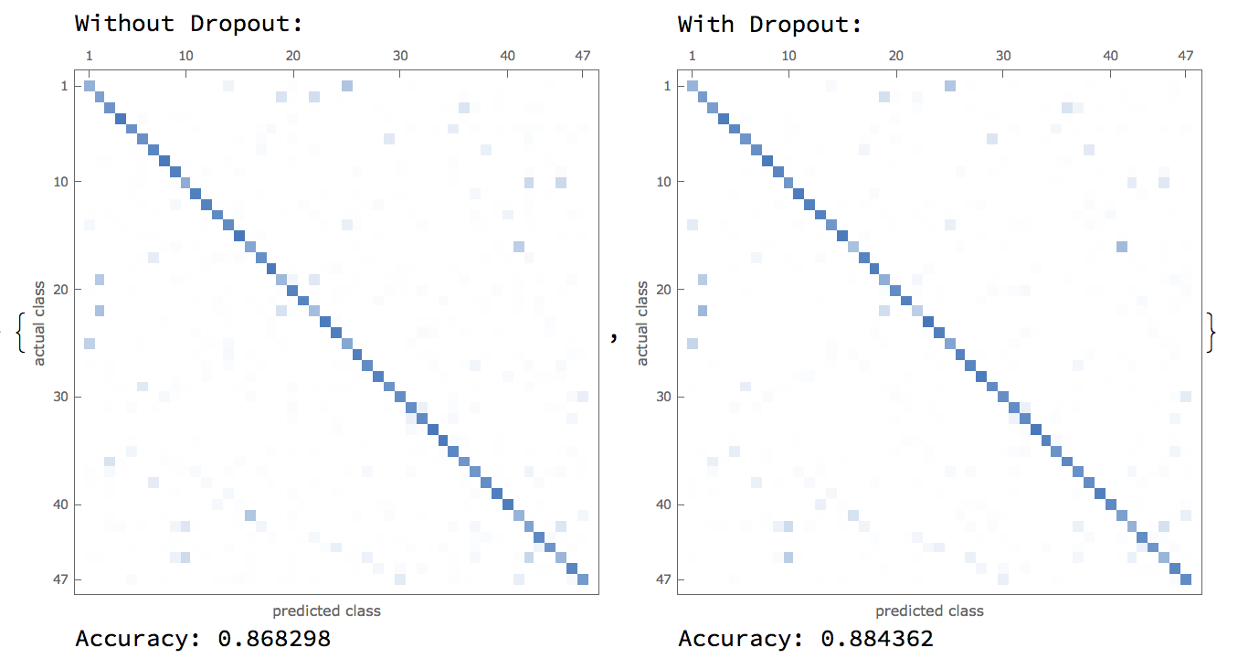 Furthermore, research into convolutional neural nets revealed two optimizers that are currently industry-standard, which were the ADAM and SGD optimizers. A comparison between these two optimizers are shown below:
  With this, it was revealed that for our purposes, an SGD optimizer used with a DropoutLayer[] was the best combination in terms of neural network accuracy.
Code used to train network:
balancedTrainingData = cvtIndex2Train[indexed];
convolutionalNeuralNet = NetInitialize[convolutionalNeuralNet];
trained =
 NetTrain[convolutionalNeuralNet, balancedTrainingData,
  Method -> "SGD"]
Evaluating Probabilities of Outputs
Obviously, it is difficult for a neural network to return 100% probability for a single class for every image input. For each classification, there is a probability value associated with it. However, many probability values (especially those that are small) aren't that useful.
returnTopPossible[input_Image, int_Integer] :=
 Table[{cvtCode2Char[#[[n, 1]]], #[[n, 2]]}, {n, 1, int}] &[
  Flatten /@
   List @@@ Normal@ReverseSort[net[input, "Probabilities"]][[;; int]]]
The returnTopPossible function can help to return the top few probabilities based on a given input. 
Now, it is important to note that probability values range from 0~1, so 0.92 will indicate 92%. The reason why we limit the probability outputs to a few values is because there is only a minimal chance that the neural net processed an image correctly with only an output probability of, lets say, 1/10000.
Testing on Images Not from EMNIST
While EMNIST provides diverse data, still the format is similar, so we decided to test the neural network on other external images obtained from the internet.
testImage2 =
     ColorConvert[
       ImageResize[
        Import["/Users/danielshin/Desktop/test.png"], {28, 28}],
       "Grayscale"] // ColorNegate;
Thread[testImage2 -> returnTopPossible[testImage2, 5]]
The output of the testing processed was quite satisfying: 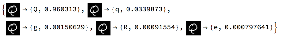
As shown, the neural network outputted a confidence score of the 96% for the image to be the capital letter "Q".
The reason we converted the image to grayscale, and then performed a color negate was because the EMNIST dataset is comprised of images that are white in a black background. Therefore, the results of the neural network is vastly inconsistent when we input an image with a white background.
Finding Characters in a Word
The neural network we made previously is confined to detecting characters that are confined specifically to an image of size 28x28. But what if there are multiple letters in an image, and the image is not in the appropriate dimensions to be reduced? In this section, we will be creating methods to detect multiple characters out of a single image.
For instance, if we have the image down below, our current neural network can't detect it properly.

First of all, we extract each letter from the image using functions such as Morphological Components. We created a function called selectChar which outputs a list of images that are single characters extracted from an image of a word.
selectChar[image_, negate_: True] := Module[
  {binarized, length},
  binarized =
   If[negate, ColorNegate[Binarize[image]], Binarize[image]];
  length =
   Length[Union[Flatten[MorphologicalComponents[binarized]]]] - 1;
  Table[SelectComponents[binarized, #Label == n &], {n, 1, length}]
  ]
selectChar[word]
** Note that the "negate" parameter is defaulted to True, as we assume that the image has a white background by default.
When the function is applied to the image shown above, it outputs:  However, it is evident that these words are not organized properly, so if we run the neural network on words that are the way that is the network will return "Nwe" not "New". Therefore, we need a method to organize the images from left to right. In our case, we utilized pixel positions and got the leftmost pixel coordinates to order each image.
orderFromLeft[charList_] :=
 Table[#[[i, 1]], {i, 1, Length[charList]}] &[
  SortBy[Table[{charList[[n]],
     SortBy[PixelValuePositions[charList[[n]], 1], First][[1,
      1]]}, {n, 1, Length[charList]}], Last]]
However, what about letters like "i", or "E" in this case? Letters like that have separations between the top and bottom part, but utilizing MorphologicalComponents will separate them and classify them into different components, as shown in the image below: 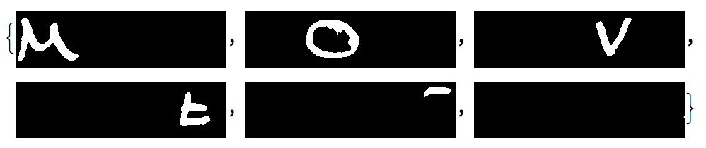
A function called checkOverlap was created to determine whether to combine components together to form a whole image:
checkOverlap[image1_, image2_] := Module[
  {overlap, imgW},
  imgW = Min[
    Max[First /@ PixelValuePositions[image1, 1]] -
     Min[First /@ PixelValuePositions[image1, 1]],
    Max[First /@ PixelValuePositions[image2, 1]] -
     Min[First /@ PixelValuePositions[image2, 1]]];
  overlap =
   Min[Max[First /@ PixelValuePositions[image1, 1]],
     Max[First /@ PixelValuePositions[image2, 1]]] -
    Max[Min[First /@ PixelValuePositions[image1, 1]],
     Min[First /@ PixelValuePositions[image2, 1]]];
  If[imgW*0.3 < overlap, True, False]]
Still, we can't just feed these images to the neural network. The network chain was defined to take in an image that is of size 28x28. Therefore, we need to find a way to trim and reshape the images into a 28x28 box.
reshape[image_] := Module[
  {h, w, trimmed, targetH = 26, targetW = 26, fw, fh, scale,
    resizedImage, rectangle},
  trimmed = ImageCrop[image];
  {w, h} = ImageDimensions[trimmed];
  fw = w / targetW;
  fh = h / targetH;
  scale = Max[fw, fh];
  resizedImage =
   ImageResize[trimmed, {Max[w/scale, 1], Max[h/scale, 1]}];
  rectangle = Image[Table[Table[0, 28], 28]];
  ImageCompose[rectangle, resizedImage, {Center}]
  ]
Finally, there were instances where images contain noise. These random particles were also extracted from morphological components and were resized. To filter these noise out, we decided to compare the black pixel to white pixel ratio. Assuming that each noise is a circle, the ratio would be 0.25 Pi : 1, which is about 615 pixels per 784.
filter[images_] :=
 Select[Table[
   If[Length[PixelValuePositions[images[[n]], 1]] < 615,
    images[[n]]], {n, 1, Length[images]}], ImageQ]
Still, we realized that by only using image processing, it was hard to get accurate results. Therefore, we decided to employ other methods such as character associations as well. Character association is basically a map of characters and their associations. For instance, "q" is almost always followed by a "u", etc.
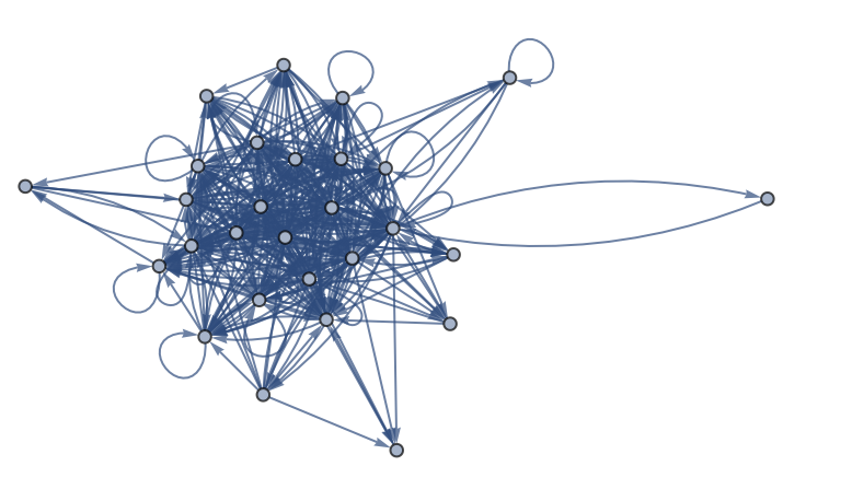
This is the character association map that was created.
Overarching Prediction Algorithm
This was the function utilized to create the final algorithm (that encompasses both the image and association probabilities)
trail[input_, weights_, edges_, negate_: True] := Module[
  {wordList, probabilityList},
  wordList = Tuples[imageProbability[moveWord, negate]];
  probabilityList = Table[outputProbability[
     Select[wordList[[n]] // Flatten, NumberQ],
     associationProbability[
      Select[wordList[[n]] // Flatten, StringQ],
      edgeWeights, withoutDuplicates
      ]], {n, Length[wordList]}];
  Select[wordList[[
       Position[probabilityList, Max[probabilityList]][[1, 1]]]] //
      Flatten, StringQ] // ToLowerCase // StringJoin
  ]
- imageProbability is a function which outputs classification probabilities of each image.
- associationProbability is a function which outputs the probabilities of word associations based on the character association map.
We combined these two probabilities to create a final output.
Conclusion & Future Works
During this project, algorithms were designed to recognize words in an image. However, results weren't exactly as satisfying as expected. The accuracy of the trained neural network was quite high, but there were some other issues as well. Using character-based relationships, the program successfully impedes consonants from following consonants, such as "Q" following "M", however the replaced vowel wasn't always quite accurate. Other attempts were made, such as adding weights as well. Only after creating weights to decrease the influence of the character association map, was the combination of the two probabilistic values yielded confident results.
There are various methods on simulating OCR. For future works, creating neural networks to input whole words and sentences will be able to create a more feasible and easy-to-use product. Furthermore, utilizing similar concepts from this project, using word-mapping (Markov chains), it might be possible to predict wrong characters or words in a sentence, and using image processing neural networks to compensate and replace certain characters.
Links


