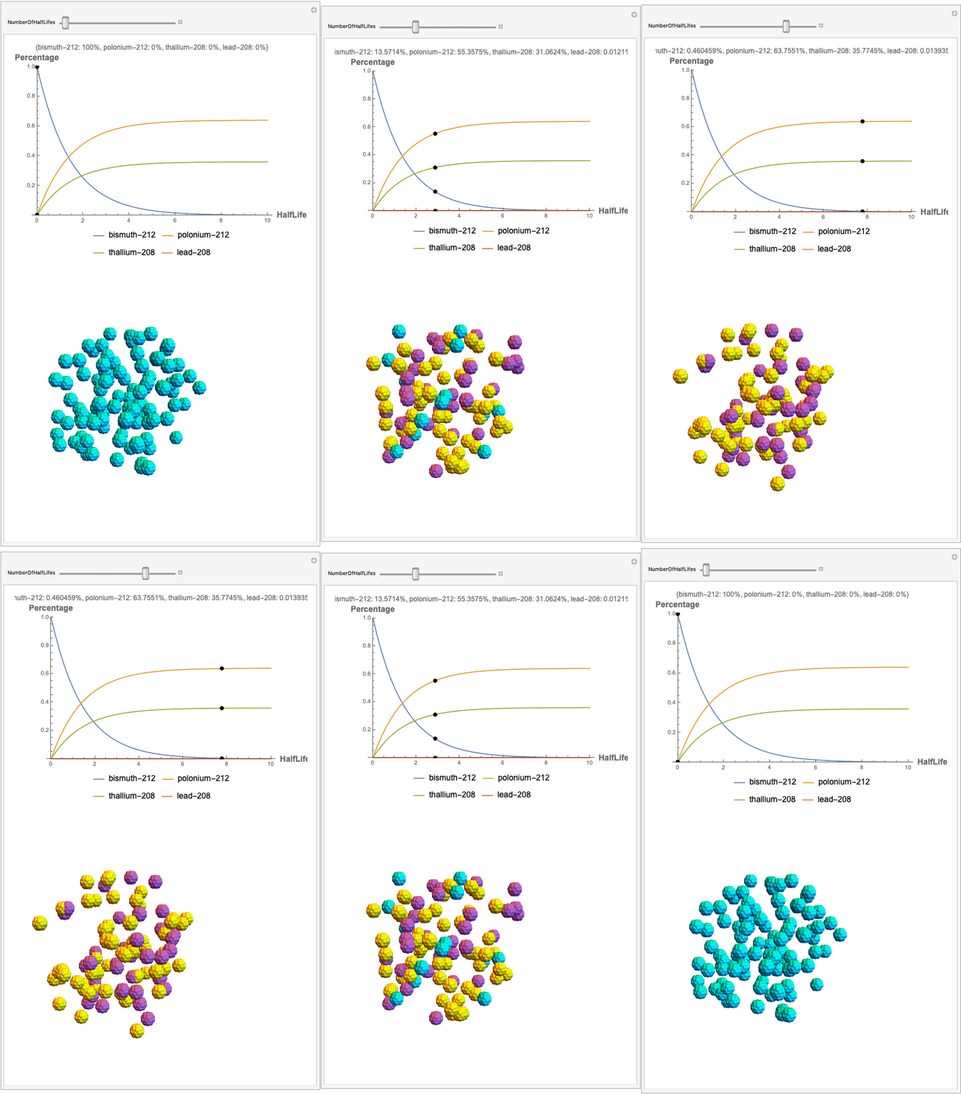
Abstract
The goal behind this project was to find a way to successfully showcase the processes behind nuclear decay reactions. Given an isotope, an algorithm was written to generate an automated interactive nuclear decay cascade chart with nodes to represent different isotopes. These nodes also provided the user with a method of visualizing the decay process by analyzing the selected isotopes' branching ratios with respect to half-life as seen above for example. Additionally, a chart was formed that provided information on all of the isotopes present in the nuclear decay cascade outputted. The user is able to use any known isotope compatible with Wolfram's IsotopeData function using natural language inputs.
I. Computing Ratios
The mathematical foundations of nuclear decay lie in the Bateman equation, proposed and solved by physicists Ernest Rutherford and Harry Bateman respectively. This model utilizes a set of differential equations in order to calculate the shape of exponential graphs that represent how the parent isotope mass gets converted, whether that be for alternative decay modes or chain decays as seen below.
$$N_{D}={\frac {N_{1}(0)}{\lambda _{D}}}\sum _{i=1}^{D}\lambda _{i}c_{i}e^{-\lambda _{i}t}\text{ where } c_{i}=\prod _{j=1,i\neq j}^{D}{\frac {\lambda _{j}}{\lambda _{j}-\lambda _{i}}}$$ While this solution describes a chain reaction for an n amount of chain reactions in a row, the program only utilizes a more specific version to describe chain reactions for specifically two-decay chains: $$ {\frac {\mathrm {d} N_{B}}{\mathrm {d} t}}=-\lambda _{B}N_{B}+\lambda _{A}N_{A0}e^{-\lambda _{A}t}$$
For the alternate decay modes, I used a set of three equations to derive the correct ratios based on the parent isotope.
- $N_{A}=N_{A0}e^{-\lambda t}$
- $N_{B}=\frac{\lambda_B}{\lambda}N_{A0} \left(1-e^{-\lambda t} \right) $
- $N_{C}={\frac {\lambda _{C}}{\lambda }}N_{A0}\left(1-e^{-\lambda t}\right) $, where $\lambda =\lambda _{B}+\lambda _{C}$.
I changed the units of the axes to create a more clear visualization that was in terms of percentages and number of half-lives rather than the number of atoms. Later, you can also notice how the branching ratios were used to construct the elegant lines displayed in the graphs.
halfLife[isotope_] :=
  IsotopeData[isotope, "HalfLife"] // QuantityMagnitude;
decayConstant[isotope_] :=
  Log[2.]/ IsotopeData[isotope, "HalfLife"] // QuantityMagnitude;
parentDecay[isotope_, t_] :=
 If[halfLife[isotope] == Infinity, 1,
  E^(-decayConstant[isotope] t*halfLife[isotope])]
parentDecay2[isotope1_Entity, t_] :=
 If[(halfLife[isotope1] == Infinity), 1, E^(-Log[2] t)]
parentDecay4[isotope1_Entity, isotope2_Entity, isotope3_Entity,
  isotope4_, t_] :=
 If[(halfLife[isotope1] == Infinity), 1, E^(-Log[2] t)]
oneDecayA[isotope_, t_] :=
 If[halfLife[isotope] == Infinity, 0,
  1 - E^(-decayConstant[isotope] t*halfLife[isotope])]
oneDecayB[isotope1_, x_, t_] :=
 IsotopeData[isotope1, "BranchingRatios"][[x]]*(1 - E^(-Log[2] t))
II. Generating Graphics
There are three major decay patterns that are demonstrated in the program. The first one is one parent radionuclide decaying to two daughter nuclides, another is one parent radionuclide decaying to three daughter nuclides, and the final one models a nuclear decay. We can use the code for the second one as an example to show how the graphic is formed.
decayChart3[isotope_] := Manipulate[
     Style[Row[{
        Module[{
          y = parentDecay2[isotope, NumberOfHalfLifes],
          z = oneDecayB[isotope, 1, NumberOfHalfLifes],
          w = oneDecayB[isotope, 2, NumberOfHalfLifes],
          x = oneDecayB[isotope, 3, NumberOfHalfLifes]},
         Plot[{
           parentDecay2[isotope, t],
           oneDecayB[isotope, 1, t],
           oneDecayB[isotope, 2, t],
           oneDecayB[isotope, 3, t]}, {t, 0, 10},
          PlotRange -> {0, 1},
          PlotLegends ->
           Placed[{"Parent Isotope", "Child Isotope1", "Child Isotope2",
             "Child Isotope3"}, Below],
          Epilog -> {PointSize[Large], Point[{NumberOfHalfLifes, y}],
            Point[{NumberOfHalfLifes, z}], Point[{NumberOfHalfLifes, w}],
             Point[{NumberOfHalfLifes, x}]},
          PlotLabel -> {"Parent Amount: " <> ToString@ (y*100) <> "%",
            "Child1 Amount: " <> ToString@ (z*100) <> "%",
            "Child2 Amount: " <> ToString@ (w*100) <> "%",
            "Child3 Amount: " <> ToString@ (x*100) <> "%"},
          ImageSize -> 500]],
        blueList[[
         Round[100*parentDecay2[isotope, NumberOfHalfLifes]] + 1]],
        yellowList[[
         Round[100*oneDecayB[isotope, 1, NumberOfHalfLifes]] + 1]],
        purpleList[[
         Round[100*oneDecayB[isotope, 2, NumberOfHalfLifes]] + 1]],
        greenList[[
         Round[100*oneDecayB[isotope, 3, NumberOfHalfLifes]] + 1]],
        }],
      ImageSizeMultipliers -> {0.34, 0.34}],
     {NumberOfHalfLifes, 0, 10}]]
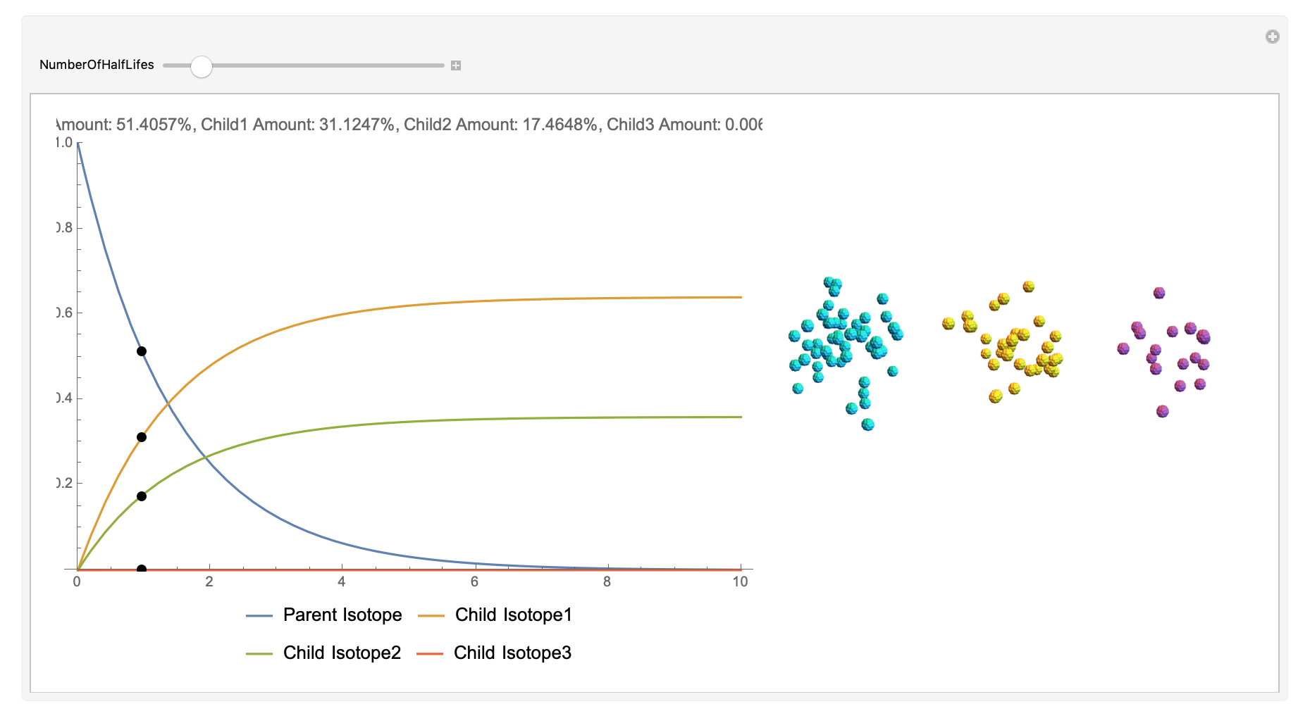
Here, we can see the code behind the plots. However, still, need to still generate the graphics that represent the masses behind each of the particles. The different colors represent the parent radionuclides and the daughter nuclides, with the protons and neutrons of the isotopes represented by a collection of spheres at the vertices of dodecaisocahdroncompounds in a three-dimensional volume.
vc = PolyhedronData["DodecahedronIcosahedronCompound", "Vertices"];
molecule1 = {RGBColor[0, 68, 105],
     GraphicsComplex[#, Table[Sphere[i], {i, Length[#]}]]} &@vc;
molecule2 = {RGBColor[120, 48, 0],
     GraphicsComplex[#, Table[Sphere[i], {i, Length[#]}]]} &@vc;
molecule3 = {Hue[0.81, 0.5, 0.84],
     GraphicsComplex[#, Table[Sphere[i], {i, Length[#]}]]} &@vc;
molecule4 = {Hue[0.28, 0.85, 0.79],
     GraphicsComplex[#, Table[Sphere[i], {i, Length[#]}]]} &@vc;
The shapes were then placed in these boxes at random. Because I chose to analyze the amounts in term of percentages, I made a list of 100 elements for each color, ranging from graphics with isotopes of each color in increments ranging to a hundred.
isotopeParent[x_] :=
  Graphics3D[
   Table[GeometricTransformation[#, transform[{0, 0, 0}]] &@
     molecule1, x], Boxed -> False, PlotRange -> {-30, 30}];
isotopeChild[x_] :=
  Graphics3D[
   Table[GeometricTransformation[#, transform[{0, 0, 0}]] &@
     molecule2, x], Boxed -> False, PlotRange -> {-30, 30}];
isotopePurple[x_] :=
  Graphics3D[
   Table[GeometricTransformation[#, transform[{0, 0, 0}]] &@
     molecule3, x], Boxed -> False, PlotRange -> {-30, 30}];
isotopeGreen[x_] :=
  Graphics3D[
   Table[GeometricTransformation[#, transform[{0, 0, 0}]] &@
     molecule4, x], Boxed -> False, PlotRange -> {-30, 30}];
Now, the plot generator will output the images correlating to the percentage at a given half-life. Using the example from before, the diagram for a one-parent to a three-child relationship can be modeled as seen below for Bismuth-212: 
III. Charts
Relation Graphs
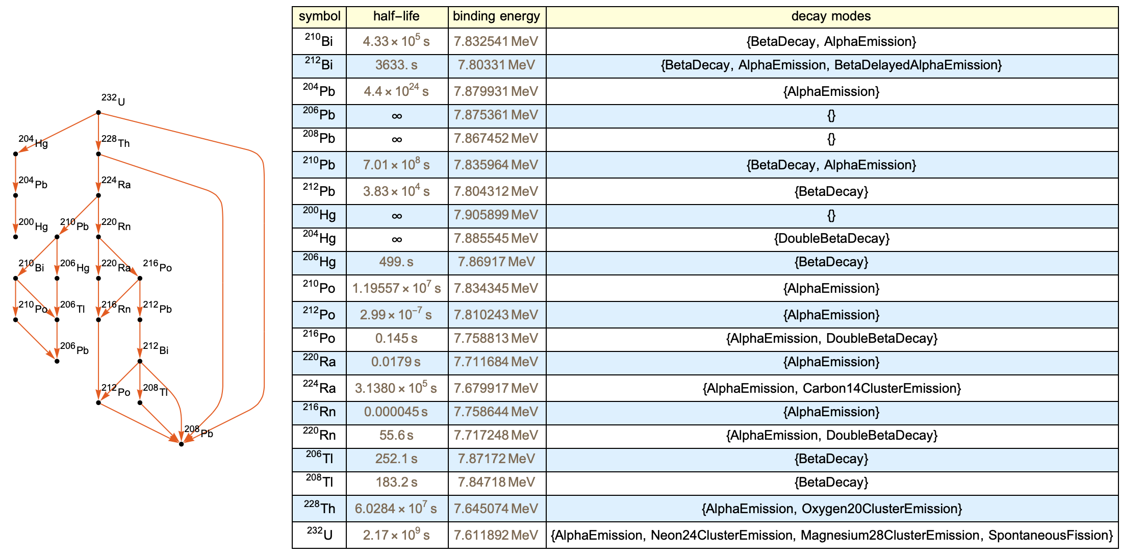
A relation graph can be used to represent the decay chains. This is because the Wolfram language has the ability to automatically construct charts that have vector connections with the parent isotopes and their respective child isotopes. Writing functions that utilize the Wolfram IsotopeData function helped to write functions that could be used by each node to identify the children isotopes.
DaughterNuclides[s_List] :=
  DeleteCases[
   Union[Apply[Join,
     Map[IsotopeData[#, "DaughterNuclides"] &,
      DeleteCases[s, _Missing]]]], _Missing];
ReachableNuclides[s_List] :=
  FixedPoint[Union[Join[#, DaughterNuclides[#]]] &, s];
DaughterNuclidesQ[s1_,  s2_] := (s1 =!= s2 && MemberQ[DaughterNuclides[{s1}], s2]);
children[x_Entity] := ReachableNuclides[{x}]
getSymbol[isotope_] := IsotopeData[isotope, "Symbol"]
decaySymbols[isotope_] := getSymbol[#] & /@ children[isotope]
Next, I created an autogenerating vertex label system which takes an isotope makes connections between different nodes.
makeVertexLabels[isotope_] :=
 Table[children[isotope][[i]] -> decaySymbols[isotope][[i]], {i, 1,
   Length@decaySymbols[isotope]}]
By combing these methods, the below function makes the decay chart with any given isotope in the Wolfram database.
RelationGraph[DaughterNuclidesQ, children[isotope],
 Sequence[VertexLabels -> makeVertexLabels[isotope],
  PlotRangePadding -> 0.65, ImageSize -> 300,
  PlotTheme -> "Scientific"]]
Information Chart
The information chart works along with the relation tree in the same overall function. It is a table that uses the IsotopeData function to post decay statistics and type for all child isotopes of the parent molecule.
makeChart[isotope_] :=
 Text[Grid[
   Prepend[Table[
       IsotopeData[#,
        prop], {prop, {"Symbol", "HalfLife", "BindingEnergy",
         "DecayModes"}}] & /@ children[isotope], {"symbol",
     "half-life", "binding energy", "decay modes"}], Frame -> All,
   Background -> {None, {{{LightBlue, White}}, {1 -> LightYellow}}}]]
The below function puts everything together and generates an output. We can use the Uranium-232 as an example isotope entity.
makeDecayGraphSample[isotope_] :=
 Row[{RelationGraph[DaughterNuclidesQ, children[isotope],
    Sequence[VertexLabels -> makeVertexLabels[isotope],
     PlotRangePadding -> 0.65, ImageSize -> 300,
     PlotTheme -> "Scientific"]], makeChart[isotope]}]

IV. Button Integration
The buttons at the place of the nodes serve to integrate part two with the rest of the program. I made a function that looks at each isotope and then decides what type of chart it should be used it depending on the number of children isotopes.
graphf[isotope_] :=
 If[Length@DeleteMissing@IsotopeData[isotope, "DaughterNuclides"] ==
   1, decayChart4[isotope],
  If[Length@DeleteMissing@IsotopeData[isotope, "DaughterNuclides"] ==
    2, decayChart2[isotope],
   If[Length@DeleteMissing@IsotopeData[isotope, "DaughterNuclides"] ==
      3, decayChart3[isotope],
    Return[""]]]]
vertexGenerate[{xc_, yc_}, vertex_, {w_, h_}] :=
  Inset[
   Button[
    vertex,
    currentChart = graphf[vertex]],
   {xc, yc}];
Using this, I modified the original relationship graph function to depict the updated vertexGenerate function to combine all the different sections of the code in one function.
makeDecayGraph[isotope_] := Module[{graph, currentChart = {}},
  vertexGenerate[{xc_, yc_}, vertex_, {w_, h_}] :=
   Inset[
    Button[
     vertex,
     currentChart = graphf[vertex]],
    {xc, yc}];
  graph = RelationGraph[DaughterNuclidesQ, children[isotope],
    Sequence[VertexLabels -> None,
     PlotRangePadding -> 0.65, ImageSize -> 800,
     PlotTheme -> "Scientific",
     VertexShapeFunction -> vertexGenerate]];
  Column[{graph, Dynamic[currentChart]}]
  ]
This resulted in a final output that, for demonstration, inputs the Uranium-232 isotope (with the Bismuth-212 button pressed).

Future Extensions
Some possible extensions that this program could have is making n-chain reaction functions. The program currently doesnt fully exploit the differential recursive functions outlined in the Bateman model. This way, for any potential given chain process, all the successive decays would be calculated. The graphical representations of the decay shown with the molecules behavior over a certain number of half-lives could be updated to showcase a variety of more animations that help explain the behavior of the decay pattern.
Github
https://github.com/srangan24/WSS-Template
 Attachments: