Introduction
Many years ago I used to assist my professor in teaching Inorganic Chemistry for beginners. Every now and then when talking about orbitals somebody asked : "I understand $d(x,y)$ and so, but what are the reasons for these funny names $d( 2 z^2 - x^2 - y^2 )$ and $d( x^2 - y^2 )$ for the other orbitals?"
I found Schroedinger's equation too complicated for beginners and I thought about a "geometrical" explanation. This is given in the attached notebook.
Please note that the plots need quite a lot of memory. This may be reduced by enclosing the plot-commands in Rasterize[...].
I wish to thank Henrik Schachner for proof-reading and for correcting numerous typos.
Some Thoughts concerning Atomic Orbitals
The following statements are to be considered as plausibility-considerations concerning the "form" of atomic orbitals. The correct quantum mechanical functions are not given, but, if one accepts the idea of nodal surfaces and their influence on energy, it is shown how the images and notations given in textbooks might have their origins.
Bohr
Bohr assumed the electron to be a point-like particle with mass $m_e$ and charge - 1 or rather - e which interacts with an atomic nucleus with mass $m_p$ and charge + 1 or + e according to Coulomb's Law. At this stage orbits and energies whatsoever are possible. To confine the orbits Bohr postulated that only non-fractional (integral?) multiples of Planck's constant were allowed for the values of angular momentum:
$L = m_e (r^2) ? = n h $
yielding a model with discrete orbitals and energies.
The success was overwhelming.
Not only the series of spectral lines of hydrogen could be precisely calculated but as well the empirically obtained so called Rydberg's Constant was obtained with high precision using the parameters of the model:
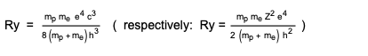
But despite numerous refinements (inclusion of the nucleus in the so called reduced mass (as already done in Ry), admittance of elliptical orbits and inclusion of relativistic effects) it was not possible to describe more complicated effects. One got stuck.
Quantum Mechanics
In the time after Bohr the conviction grew that the electron wasn't a particle, but instead its negative charge was somehow distributed around the atomic nucleus. And furthermore there were different distributions linked to different energies. These ideas lead to a theory which nowadays is called Quantum Mechanics.
See as well:
"J.J. Thomson got the Nobel prize for demonstrating that the electron is a particle. George Thomson, his son, got the Nobel prize for demonstrating that the electron is a wave" in B. Povh, M. Rosina, Streuung und Strukturen, Springer 2002, S. 15. (ISBN 3 540 42887 9)
similar in P.W. Atkins, Molecular Quantum Mechanics, Clarendon Press Oxford 1970, S. 16, footnote. (ISBN 0 19 855129 0)
And in [ Richard Feynman, winner of the Nobel Prize concludes : "It is neither particle nor wave...." , Silvia Arroyo Camejo, Skurrile Quantenwelt, p. 98 (ISBN 978-3-596-17489-8) ]
These charge-distributions can be described by functions having a certain periodic character (waves!) in such a way, that the square of such a function is proportional to the charge density.
Why the square? Well, it is always zero or greater than zero as it is to be expected of a charge distribution.
s - Orbital
The most simple function for a spherical symmetric charge distribution is a function depending only on the distance from the origin. This function should approach zero quick enough to yield a finite radius of the atom, even it is sort of impossible to say exactly what that is.
In a system of coordinates:
null = {0, 0, 0};
ex = {1, 0, 0};
ey = {0, 1, 0};
ez = {0, 0, 1};
we write for the function looked after
s[x_, y_, z_] := Exp[-(x^2 + y^2 + z^2)]
This is NOT the function given by Quantum Mechanics, this were  but the function chosen here is more convenient if calculations should be made and is well appropriate for further discussions..
Let's proceed to look at the s - Orbital. But what does that mean: look at the s - Orbital?
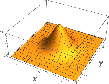
Here we have a function of three variables, and to draw a picture one must have a space of four dimensions, which is not available. But one could fix one coordinate, z = 0 say, and then plot the function for variable x and y perhaps in the following way
Plot3D[s[x, y, 0], {x, -3, 3}, {y, -3, 3}, PlotRange -> All, AxesLabel -> {Style[x, Large, Bold], Style[y, Large, Bold]}]
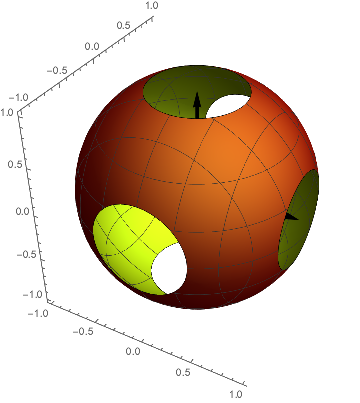
Or we chose an arbitrary value the function should attain, say $=.3$, and look for all points $( x, y, z )$ which yield this value. This is, what usually is shown in textbooks: a surface on which the function yields this number. And even more precise we see a projection of this object onto a two-dimensional page of paper.
As our function depends only on $r^2$ we expect a spherical entity as shown here. The plot region is a bit too small, so that there are holes in the surface and we can peek into it. With a tiny bigger plot region the surface were closed.
achsen[f_] :=
 Graphics3D[{Thickness[.01], Arrow[{null, f ex}], Arrow[{null, f ey}],
    Arrow[{null, f ez}]}, Boxed -> False]
Clear[p0];
gg = 1.;
p0 = ContourPlot3D[
   s[x, y, z], {x, -gg, gg}, {y, -gg, gg}, {z, -gg, gg},
   Contours -> .3, ContourStyle -> FaceForm[Red, Yellow],
   Boxed -> False, Mesh -> {5, 5}];

Show[p0, achsen[gg]]
p - Orbitals
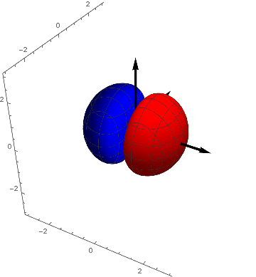
When the charge distribution is confined to smaller regions the total energy will rise ( this is not the case however, as theory (and experiment) shows for the hydrogen-atom where s- , p- , d- orbitals and so on have all the same energy). An idea to compress the charge distribution could be to introduce a region in space where the function attains a value of zero. That could be achieved in lots of ways, e.g. multiplying s with $x$. Or with $y$, or with $z$. If $x = 0$, then the whole thing is zero. In this way so called nodal planes are introduced, onto which the function disappears. We get three new functions which have the same energy due to the fact, that the axes of the coordinate-system are principally not to be discerned, the new functions are degenerate. Here the so called $p_x$ - Orbital is shown
$p_x = x$ $s[x, y, z]$
with $p_x = ± 0.04$.
px = ContourPlot3D[x s[ x, y, z], {x, -3, 3}, {y, -3, 3}, {z, -3, 3},
   Contours -> {{.04, Red}, {-.04, Blue}}, Boxed -> False,
   Mesh -> {5, 5}];
Show[px, achsen[3]]
The $p_y$ - Orbital looks alike (and of course $p_z$):
py = ContourPlot3D[y s[ x, y, z], {x, -3, 3}, {y, -3, 3}, {z, -3, 3},
   Contours -> {{.04, Red}, {-.04, Blue}}, Boxed -> False,
   Mesh -> {5, 5}];
Show[py, achsen[3]]
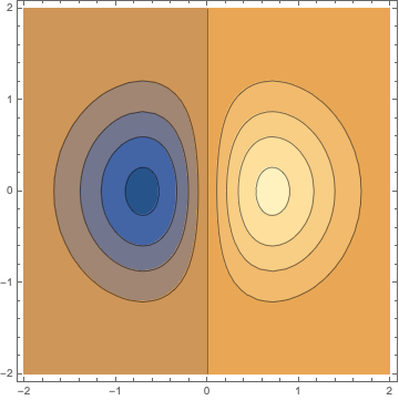
This may be shown as contour-plot in two dimensions. The contours evoke the impression that the charge distribution is compressed.
ContourPlot[x s[x, y, 0], {x, -2, 2}, {y, -2, 2}]
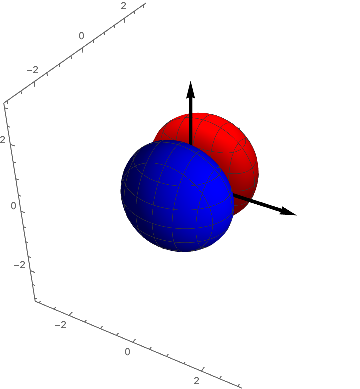
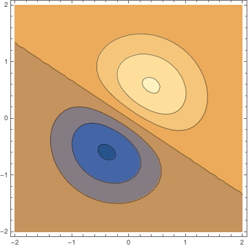
An interesting observation is that the orbital must not point in the direction of an axes. By "mixing" two functions another function with different behaviour is obtained, shown here for $0.4 p_x + 0.6 p_y$
ContourPlot[(.4 x + .6 y) s[x, y, 0], {x, -2, 2}, {y, -2, 2}]
d - Orbitals
The next step. To confine the charge distribution even further we introduce a second nodal plane. But how? For the p-orbitals we have multiplied s with x and so on. That suggests the multiplication with products constructed from x, y and z. That is easy and gives the  ,
,  and
and  - Orbitals, hence three functions or orbitals.
pxy = ContourPlot3D[ x y s[ x, y, z], {x, -3, 3}, {y, -3, 3}, {z, -3, 3},
   Contours -> {{.02, Red}, {-.02, Blue}}, Mesh -> {5, 5}];
Show[pxy, achsen[3]]
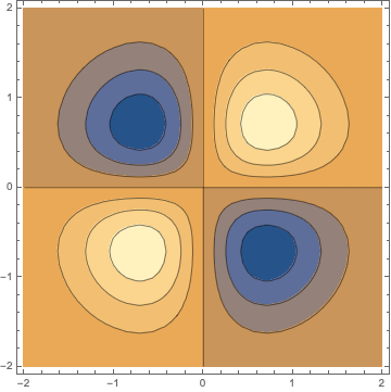
In two dimensions as above this looks like
ContourPlot[(x y) s[x, y, 0], {x, -2, 2}, {y, -2, 2}]
and as further example
pyz = ContourPlot3D[
   y z  s[ x, y, z], {x, -3, 3}, {y, -3, 3}, {z, -3, 3},
   Contours -> {{.02, Red}, {-.02, Blue}}, Boxed -> False,
   Mesh -> {5, 5}];
Show[pyz, achsen[3]]
But what shall we do with the three remaining products x x, y y and z z? These obviously give only one nodal plane, namely for $x = 0$, $y = 0$ and $z = 0$.
One could of course try linear combinations like
$d1 = ( x + y ) ( x - y ) = x^2 - y^2$
$d2 = ( x + z ) ( x - z ) = x^2 - z^2$
$d3 = ( y + z ) ( y - z ) = y^2 - z^2$
so d1 is zero for $x = y$ and $x = -y$ and we arrive at three further functions with two nodal planes. But - these three function are not independent !
We have $d3 = d2 - d1$
so that essentially only two functions with the desired number of nodal planes remain. Therefore there are altogether five d - orbitals
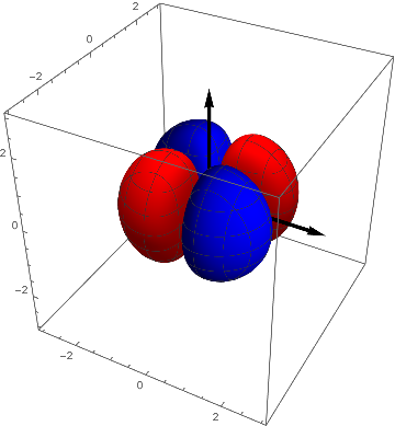
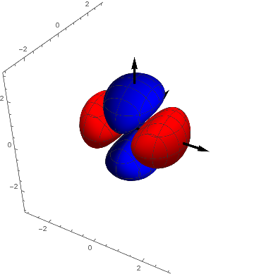
p1 = ContourPlot3D[(x^2 - y^2)  s[ x, y, z], {x, -3, 3}, {y, -3,
    3}, {z, -3, 3}, Contours -> {{.05, Red}, {-.05, Blue}},
   Boxed -> False, Mesh -> {5, 5}];
Show[p1, achsen[3]]
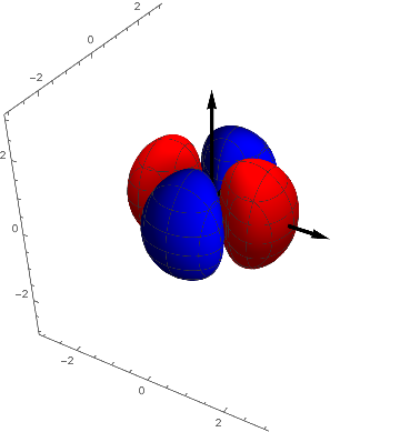
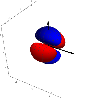
The remaining functions f2 and f3 look like
p2 = ContourPlot3D[( x^2 - z^2)  s[ x, y, z], {x, -3, 3}, {y, -3,
    3}, {z, -3, 3}, Contours -> {{.05, Red}, {-.05, Blue}},
   Boxed -> False, Mesh -> {5, 5}];
Show[p2, achsen[3]]
p3 = ContourPlot3D[( y^2 - z^2)  s[ x, y, z], {x, -3, 3}, {y, -3,
    3}, {z, -3, 3}, Contours -> {{.05, Red}, {-.05, Blue}},
   Boxed -> False, Mesh -> {5, 5}];
Show[p3, achsen[3]]
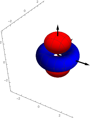
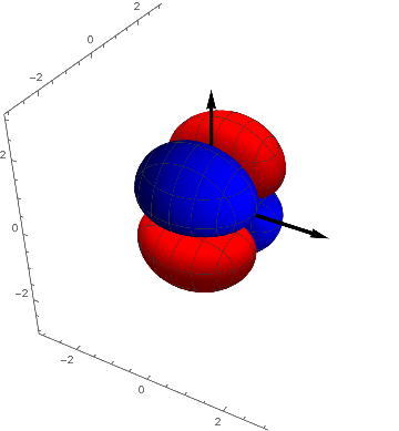
It can be seen that they are transformed into each other by a rotation of 90º around the $z-axis$. They are in a certain sense equivalent and we combine them by forming their average ( the here used multiplication with $-1$ yields the textbook-representation) and we have an explanation for the name $(2 z^2 - x^2 - y^2 )$ - orbital for this function.
$d5 = - ( d2 + d3 ) / 2 = z^2- ( x^2 + y^2) / 2 = ( 2 z^2 - x^2 - y^2 ) / 2$
p4 = ContourPlot3D[(  2 z^2 - x^2 - y^2)  s[x, y, z], {x, -3,
    3}, {y, -3, 3}, {z, -3, 3},
   Contours -> {{0.1, Red}, {-0.1, Blue}}, Boxed -> False,
   Mesh -> {5, 5}];
Show[p4, achsen[3]]
f - Orbitals
For f-orbitals one more nodal plane is needed. One could think of using for example
f1 = x y z
f2 = x (x + y)( x - y)
f3 = x (x + z) (x - z)
f4 = y (y + x) (y - x)
f5 = y (y + z) (y - z)
f6 = z (z + x) (z - x)
f7 = z (z + y) (z - y)
f8 = x (z + y) (y - z)
f9 = y (x + z) (x - z)
f10= z (x + y) (x - y)
These are ten functions with three nodal planes. But it turns out that only seven of these are independent. Therefore there are seven f - orbitals.
But to find them is left to the reader.
 Attachments:


