Testing the concept:

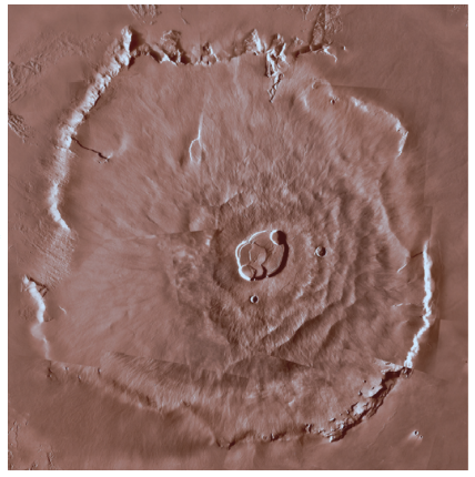
To test and calibrate the method, I used an example (not from a moon): Olympus Mons on Mars, and highlighted areas of the image that stand out as bright white areas, enhanced by code and subsequently inverting the color:

olympus = 
 GeoGraphics[Entity["SolarSystemFeature", "OlympusMonsMars"], 
  GeoRange -> Quantity[200, "Miles"]]

ColorNegate[
 ChanVeseBinarize[
  ColorConvert[ImageAdjust[olympus, {0, 0.8, 0.8}, {0.5, 1}, {0, 1}], 
   "Grayscale"], Gray]]

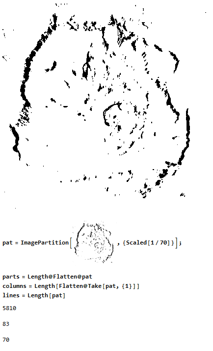
After dividing the image (above) into many small regions (5810 smaller images), I characterize each piece with its values (ImageData) using the following line:

cd = Parallelize[
   Table[Table[
     N[Mean@Flatten@ImageData[((Take[pat, {vv}][[1]])[[uu]])]], {uu, 
      1, 83}], {vv, 1, 70}]];

Then I made Mathematica choose regions with average data values with a specific degree of pixels to generate red dots that will be used to mark the regions (it was noted that the method has limitations caused mainly by the size of the smaller regions, requiring a lot of memory and processing, but positively had a relative accuracy):

ur = ImageAssemble[
  Parallelize[
   Table[Table[
     If[((cd[[v]])[[u]]) < 0.85, 
      ImageCompose[((pat[[v]])[[
         u]]), {Graphics[{PointSize[Large], Red, Point[{0, 0}]}]}], 
      ImageCompose[((pat[[v]])[[
         u]]), {Graphics[{PointSize[Tiny], Opacity[0], 
          Point[{0, 0}]}]}]], {u, 1, 83}], {v, 1, 70}]]]

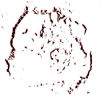
ColorReplace[ur, Black]

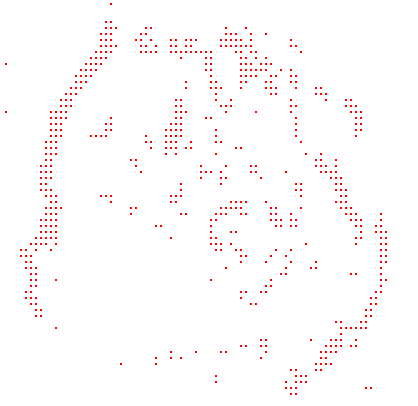
Now testing with the original Olympus Mons image (with 5810 divisions and marking bright areas for: brightness > 0.67), the code for partition the image and selecting data values to mark light areas:

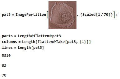
cd3 = Parallelize[
   Table[Table[
     N[Mean@Flatten@ImageData[((Take[pat3, {vv}][[1]])[[uu]])]], {uu, 
      1, 83}], {vv, 1, 70}]];

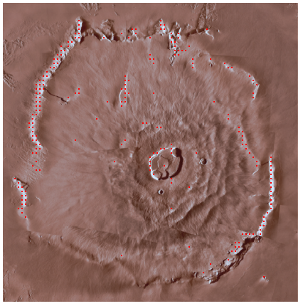
In the case of the actual image, the average pixel value must be above a specific value for selecting the required areas, the reverse of the concept test. Here is the test done with the raw image:

ur5 = ImageAssemble[
  Parallelize[
   Table[Table[
     If[((cd3[[v]])[[u]]) > 0.67, 
      ImageCompose[((pat3[[v]])[[
         u]]), {Graphics[{PointSize[Large], Red, Point[{0, 0}]}]}], 
      ImageCompose[((pat3[[v]])[[
         u]]), {Graphics[{PointSize[Tiny], Opacity[0], 
          Point[{0, 0}]}]}]], {u, 1, 83}], {v, 1, 70}]]]

Testing surface maps of moons:

Now testing the surface map of some of the solar system's moons, so we can see the previous code performance and later some variations of the same for better visualization. Below are the other examples of surface maps tested by the code, with the limit of values of the bright and the number of smaller computed areas of each image chosen for each example.

These are the basic lines of code that will be used on the surfaces:

(1) Calculates the values of each piece of the image, same code to all examples (note: set the image on the code!):

x = ImagePartition["image", {Scaled[1/70]}];
y = Parallelize[
   Table[Table[
     N[Mean@Flatten@ImageData[((Take[x, {vv}][[1]])[[uu]])]], {uu, 1, 
      70}], {vv, 1, 70}]];

(2) Generates the points and reassembles the full image. Has some variations as seen in the examples later in the post (note: choose the brightness limit value on the code!):

z = ImageAssemble[
  Parallelize[
   Table[Table[
     If[((y[[v]])[[u]]) > "brightvalue", 
      ImageCompose[((x[[v]])[[
         u]]), {Graphics[{PointSize[Large], Red, Point[{0, 0}]}]}], 
      ImageCompose[((x[[v]])[[
         u]]), {Graphics[{PointSize[Tiny], Opacity[0], 
          Point[{0, 0}]}]}]], {u, 1, 70}], {v, 1, 70}]]]

Some examples:

• Jupiter´s Moon, Ganymede:

  GeoGraphics[GeoModel -> Entity["PlanetaryMoon", "Ganymede"], 
   GeoRange -> Quantity[1500, "Miles"]]
  

Using the codes gives the following result for Ganymede (marking for brightness > 0.54):

• Jupiter´s Moon, Europa (a bright moon):

  GeoGraphics[GeoModel -> Entity["PlanetaryMoon", "Europa"], 
   GeoRange -> Quantity[1000, "Miles"]]
  

Using the codes gives the following result for Europa, which has a brighter surface (marking for brightness > 0.71):

• Jupiter´s Moon, Callisto (a dark moon):

  GeoGraphics[GeoModel -> Entity["PlanetaryMoon", "Callisto"], 
   GeoRange -> Quantity[1500, "Miles"]]
  

Using the codes, we get the following result for Callisto, which has a relatively dark surface (marking for brightness > 0.27):

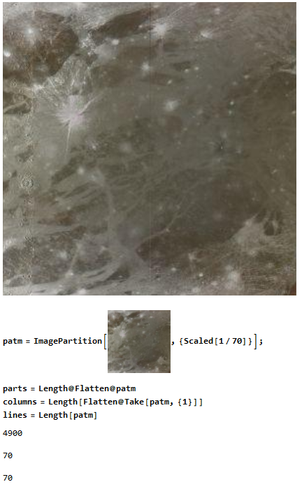
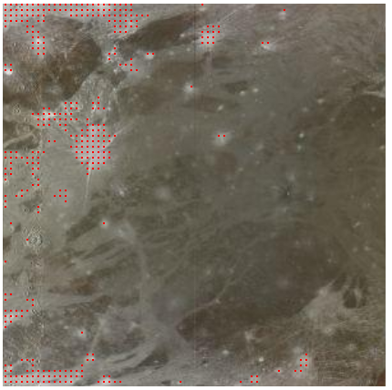
Exploring the image with dynamics:

• Saturn´s Moon, Dione:

  GeoGraphics[GeoModel -> Entity["PlanetaryMoon", "Dione"], 
   GeoRange -> Quantity[400, "Miles"]]
  

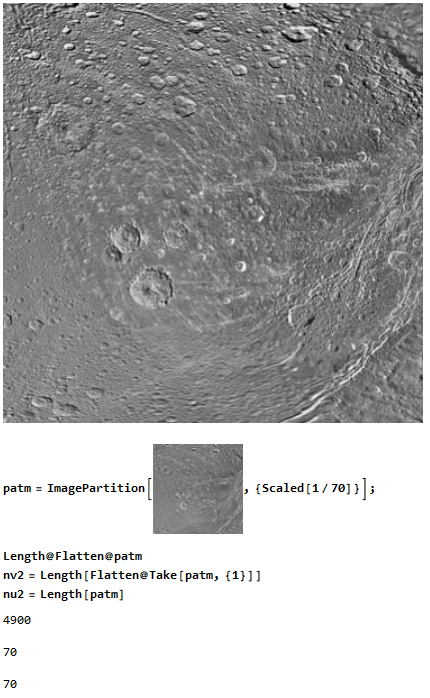
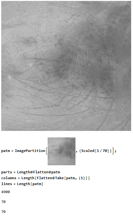
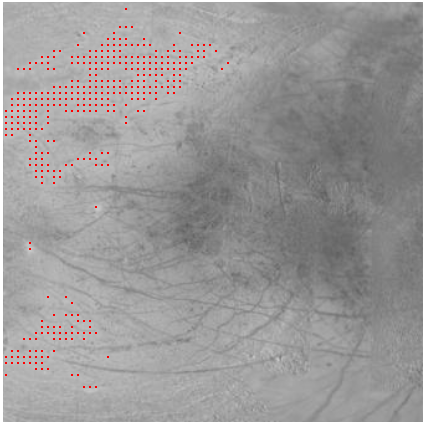
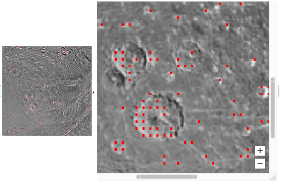
Using the first (1) code and making the second (2) code dynamic (below), I got the following result for Dione, a surface with well-distributed bright spots (marking for brightness > 0.55):

{Evaluate[
  urm = ImageAssemble[
    Parallelize[
     Table[Table[
       If[((cdm[[v]])[[u]]) > 0.55, 
        ImageCompose[((patm[[v]])[[
           u]]), {Graphics[{PointSize[Large], Red, Point[{0, 0}]}]}], 
        ImageCompose[((patm[[v]])[[
           u]]), {Graphics[{PointSize[Tiny], Opacity[0], 
            Point[{0, 0}]}]}]], {u, 1, 70}], {v, 1, 70}]]]], 
 DynamicImage[urm]}

Marking light and dark areas simultaneously:

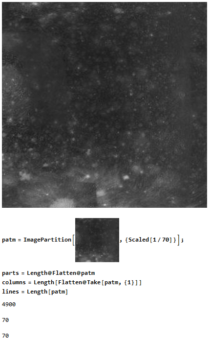
• Earth´s Moon:

  GeoImage[GeoRange -> {{-25, -5}, {45, 65}}, GeoModel -> "Moon"]
  

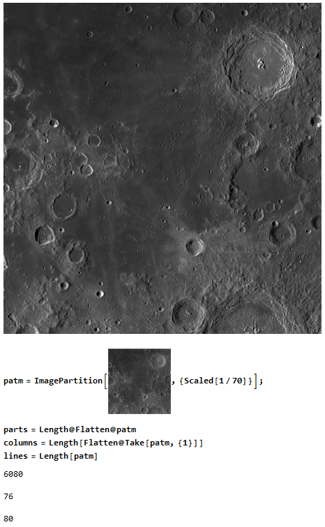
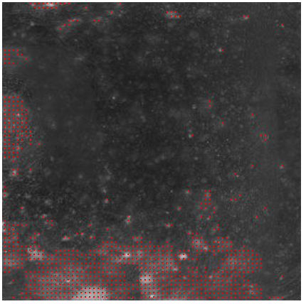
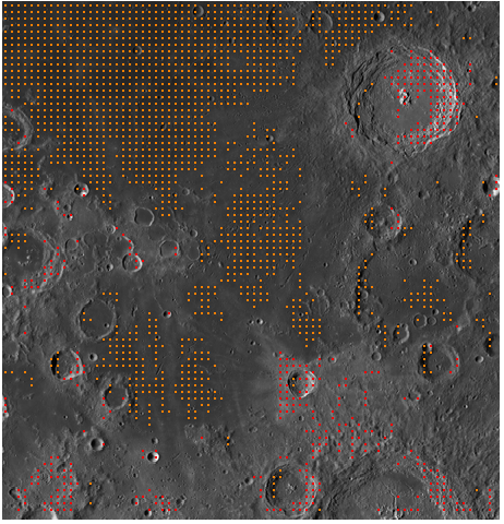
Using the first (1) code and modifying the second (2) code as below, we can mark the darkest and lightest areas on the map simultaneously. Getting the following result for Earth's Moon (marking for brightness: > 0.68 {Red}, < 0.61 {Orange}):

urm2 = ImageAssemble[
  Parallelize[
   Table[Table[
     If[((cdm[[v]])[[u]]) > 0.68, 
      ImageCompose[((patm[[v]])[[
         u]]), {Graphics[{PointSize[Large], Red, Point[{0, 0}]}]}], 
      If[((cdm[[v]])[[u]]) < 0.61, 
       ImageCompose[((patm[[v]])[[
          u]]), {Graphics[{PointSize[Large], Orange, 
           Point[{0, 0}]}]}], 
       ImageCompose[((patm[[v]])[[
          u]]), {Graphics[{PointSize[Tiny], Opacity[0], 
           Point[{0, 0}]}]}]]], {u, 1, 76}], {v, 1, 80}]]]

Viewing different intensities simultaneously:

• Jupiter´s Moon, Io (a colorful moon):

  GeoGraphics[GeoModel -> Entity["PlanetaryMoon", "Io"], 
   GeoRange -> Quantity[1000, "Miles"]]
  

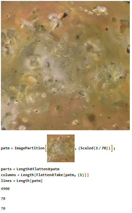
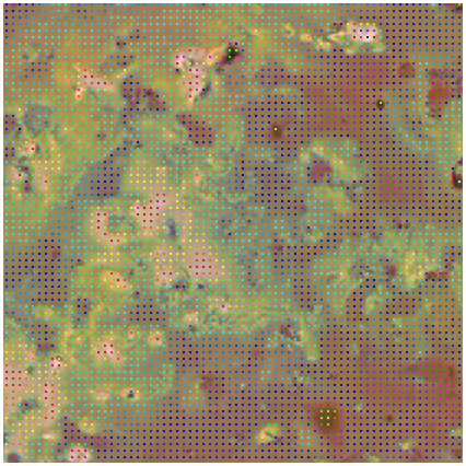
Modifying the second (2) code so that we have points with different intensities throughout the image and make them stand out with a convenient Hue function:

urm2 = ImageAssemble[
  Parallelize[
   Table[Table[
     ImageCompose[((patm[[v]])[[
        u]]), {Graphics[{PointSize[Large], 
         Hue[(150 - ((cdm[[v]])[[u]])*149)/50], Point[{0, 0}]}]}], {u,
       1, 70}], {v, 1, 70}]]]

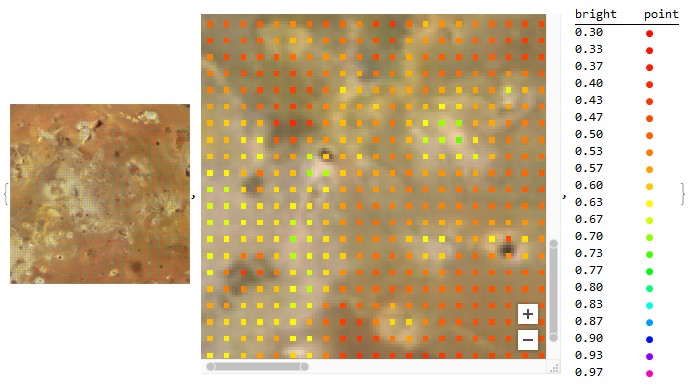
And finally, modifying again the second code (2), making the points show variations of bright with another Hue function, while dynamically exploring and labeling the intensities:

{Evaluate[
  urm = ImageAssemble[
    Parallelize[
     Table[Table[
       ImageCompose[((patm[[v]])[[
          u]]), {Graphics[{PointSize[Large], Hue[((cdm[[v]])[[u]])^4],
            Point[{0, 0}]}]}], {u, 1, 70}], {v, 1, 70}]]]], 
 DynamicImage[urm], 
 TableForm[
  Table[{N[(h/30), 2], 
    Graphics[{PointSize[Large], Hue[(h/30)^4], Point[{0, 0}]}, 
     ImageSize -> 10]}, {h, 9, 29}], 
  TableHeadings -> {None, {"bright", "point"}}]}

Thanks.